Chapter 3 Introduction to Ordinary Differential Equations

3.1 Introduction

We start by looking at how to solve a new type of equation, an ordinary differential equation. Algebraic operations such as addition and multiplication are performed on numbers, whereas the Calculus operations of differentiation and integration are performed on functions. Algebraic equations, such as $x^{2} = 25$, are solved for numbers, i.e. $x = - 5$ and $x = 5$, but differential equations are solved for functions, not numbers. Almost all of our work in this chapter deals with functions. In this section, and in any traditional course on differential equations, the symbols $x$ and $y$ are the names of functions, not independent variables. Ideally, we would write $x(t)$ and $y(t)$ in order to reinforce this point, but traditionally we just write $x$ and $y$ for brevity. Typically, $t$ is the independent variable unless otherwise stated.

We learned in algebra how to solve systems of equations with two unknowns. For example, we can easily solve the system given by: $x_1+x_2=2$ and $x_1-x_2=4$. The solution to this system of equations is $x_1=3$ ; $x_2=-1$. In this section, instead of solving for numbers, we’ll be interested in finding a function that satisfies the given relationship.

An ordinary differential equation (ODE) is an equation that includes derivatives of a single-variable function. The most basic form of an ODE is $$\frac{dy}{dt} (t)=f(t,y(t)).$$ Here, $y(t)$ is the unknown function of $t$. In words, this ordinary differential equation is satisfied by any function $y(t)$ whose derivative equals $f(t,y(t))$.

We start by looking at some examples that reinforce this fundamental concept of differential equations. Consider this ODE: $$\frac{dy}{dt} =2t.$$ Equivalently, what function $y(t)$ has a derivative equal to $2t$? An answer, $y(t)=t^2$, comes to mind quickly because we know $\frac{d}{dt}\left[t^2\right]=2t$. The function $y(t)=t^2$ is called a solution to the differential equation. However, this leads to an interesting question, “Is $y(t)=t^2$ the only solution to this differential equation?”

Consider the function $$y(t)=t^2+3$$ which has derivative
$$\frac{d}{dt}\left[t^3+3\right]=2t.$$ We see that $y(t)=t^2+3$ is also a solution to the ODE. In fact we can add any constant to $t^2$ and have a solution. Our observation leads to a general form for all possible solutions for this differential equation $$y(t)=t^2+C$$ where $C$ is any real number. This solution is called the general solution for the ODE.

Consider another differential equation. In this example, the right-hand side of the ODE contains the function we are looking for: $$\frac{dy}{dt}\left( t \right) = y\left( t \right)$$ As before, we want to know what function $y(t)$ has a derivative equal to $y(t)$? In other words, what function has a derivative equal to itself? Again, an answer, $y(t)=e^{t}$, comes to mind because we know $\frac{d}{dt}\left[e^t\right]=e^t$. We have found a solution, but have we found all the solutions? Consider the function given by $$y(t)=3e^t$$ Taking the derivative gives $$\frac{d}{dt}\left[3e^{t}\right]=3e^t.$$ Therefore, $y(t)=3e^t$ is also a solution to the differential equation. In fact, the general solution to the ODE is $y(t)=Ce^t$.

Typically, as we’ve seen, a differential equation has infinitely many solutions. The general solution for a differential equation is a description of all infinitely many solutions. The solutions are described using a parameter (arbitrary constant), in this case $C$. Choosing a specific value for $C$ gives a single function, and that function solves the differential equation. A single function that solves a given differential equation is called a specific solution to the differential equation. The phrase particular solution is often used interchangeably with specific solution in this context. In this course we’ll stick to specific solution, but the two phrases are generally interchangeable.

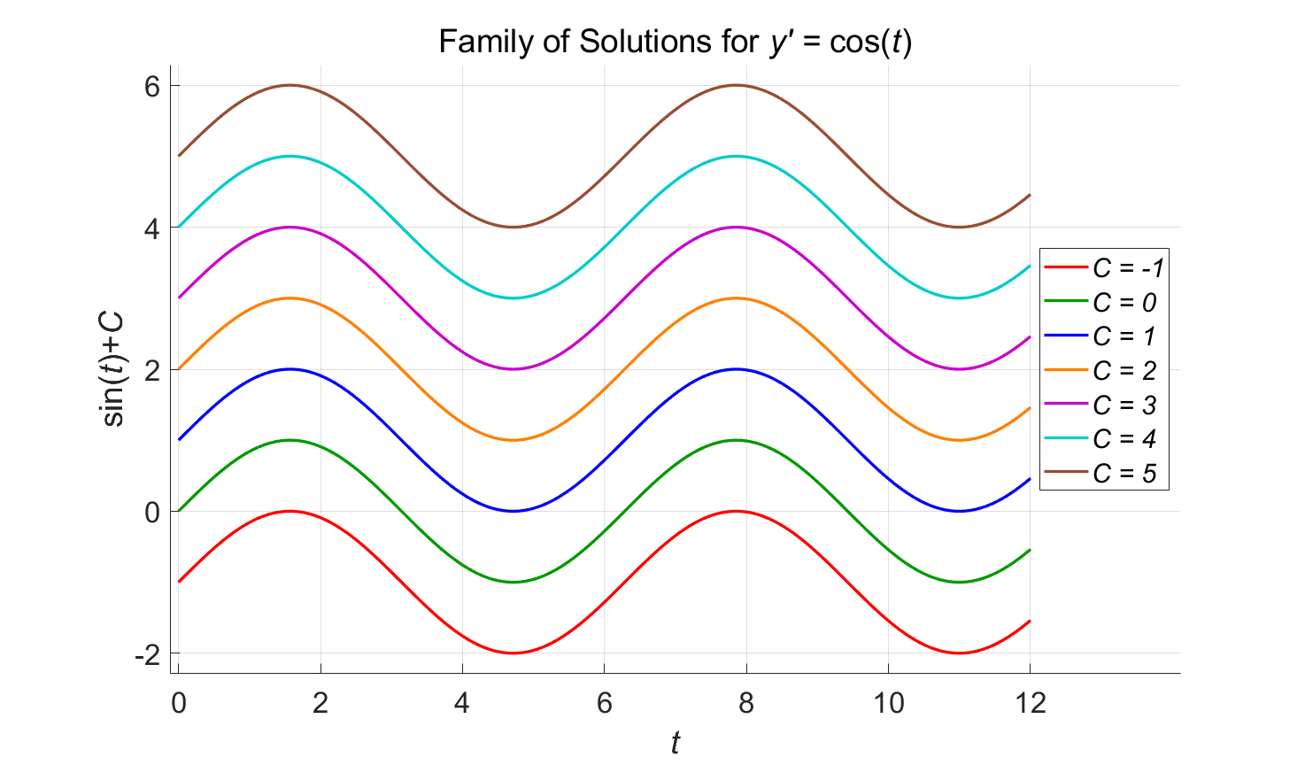
Let us investigate another example: $$\frac{dy}{dt}(t)=\cos⁡(t).$$ We address the same question as before – what function $y(t)$ has a derivative equal to $\cos(t)$? One answer is $y(t)=\sin(t)$. This function is a solution to the given differential equation. Motivated by our previous success, we look for the general solution as one of two possibilities: $$y_1(t)=C \sin(t) \text{ or }y_2 (t)= \sin(t)+C$$ where $C$ is a real number. In subsequent sections of this chapter, we will learn the methods for determining the correct solution directly. However, at this point we will simply guess and check both of the functions $y_1 (t)$ and $y_2 (t)$. Plugging a function into a differential equation to see if the function satisfies the differential equation is called verifying a potential solution.

Taking the derivatives gives $$\frac{d y_1(t)}{dt}=\frac{d}{dt}\left[C\sin(t)\right] = C\cos(t).$$

$$\frac{d y_2(t)}{dt}= \frac{d}{dt}\left[\sin(t)+C\right] = \cos(t).$$ We can see that $y_1(t)$ does not satisfy the differential equation, while $y_2(t)$ does. It turns out that we have found the general solution to the differential equation, which is $$y(t)=\sin(t)+C.$$ To demonstrate the family of solutions idea, we have a graph of several solutions that correspond with varying values of the constant $C$.

Throughout this chapter, it will be important to remember that solutions to differential equations are functions. The general solution to a differential equation is a description of infinitely many functions that all satisfy the differential equation; the description is achieved using a parameter, usually $C$. A specific solution to the differential equation is a single function.

As we have demonstrated, we can always check to see if a function is a solution to an ODE. This is called verifying a potential solution. Consider the differential equation $$y^{'}\left( t \right) = 2ty\left( t \right)$$ We seek a function $y(t)$ whose derivative equals the function itself times $2t$. Here are two candidate functions $$y_1(t)=t^2\text{ and }y_2(t)=e^{t^2},$$

and we will check these functions to see if they are solutions. To test the functions, we compute the expressions on both sides of the differential equation. It is common to write LHS to mean “the expression on the left-hand side of the equal sign”, and RHS to mean “the expression on the right-hand side of the equal sign”.

We start by testing the function $y_{1}\left( t \right) = t^{2}$. $$\begin{aligned} &\text{LHS:}\quad y_{1}^{'}\left( t \right) = 2t\\ &\text{RHS:}\quad 2ty_{1}\left( t \right) = 2t\cdot t^{2} = 2t^{3}\end{aligned}$$

The LHS and RHS are not equal, so $y_{1}\left( t \right) = t^{2}$ is not a solution to the ODE.

We repeat the process with $y_2=e^{t^2}$.

$$\begin{aligned} &\text{LHS:}\quad y_{2}^{'}\left( t \right) = 2te^{t^{2}}.\\ &\text{RHS:}\quad 2ty_2(t)=2te^{t^2}.\end{aligned}$$

Voila! We see that the LHS and RHS are equal. In other words the following is true $$y_2'(t)=2te^{t^2}=2ty_2 (t).$$ Thus, we know that $y_2=e^{t^2}$ is a solution to the differential equation.

By definition all ordinary differential equations have only a single independent variable. In this chapter we will use $t$ as our independent variable. Moreover, because the independent variable is known, we will not include the independent variable when writing the ODE’s dependent function. In the example above, we wrote $$y' (t)=2ty(t).$$ Since we know $y(t)$ is a function of $t$, the far more common way to write this ODE is $y'=2ty$. This is sloppy. However, dropping the explicit nature of the function notation is standard in the engineering and mathematics community. We must accept this standard and train ourselves to realize that the dependent function always has an independent variable.

Here are some examples showing how to verify that a function solves a given ODE.

3.1.0.1 Example #1

Determine whether or not $y_{1}\left( t \right) = \cos\left( 3t \right)$ is a solution to this ODE: $y^{'} = 3\cos\left( 3t \right)$ . $$\begin{aligned} &\text{LHS:}\quad y_{1}^{'} = \frac{d}{dt}\left[\cos\left( 3t \right)\right] = - 3\sin\left( 3t \right).\\ &\text{RHS:}\quad 3\cos\left( 3t \right).\end{aligned}$$

Sometimes it isn’t clear whether the functions on the LHS and RHS of the differential equation are the same. One way to determine whether they are the same is by plotting them. If we plot the LHS ($3\sin\left( 3t \right)$) and the RHS ($3\cos\left( 3t \right)$) we obtain the figure below. If the LHS and RHS functions were the same, their plots would overlap. These plots don’t overlap, and so the LHS and RHS functions are not the same.

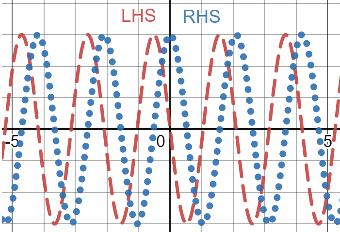
Since LHS $\neq$ RHS, the function $y_{1}\left( t \right) = \cos\left( 3t \right)$ is not a solution for $y^{'} = 3\cos\left( 3t \right)$. Notice: neither RHS nor LHS are the potential solution function, $y_{1}\left( t \right)$.

3.1.0.2 Example #2

Determine whether or not $z_{1}\left( t \right) = 2\sqrt{2t}$ is a solution to this ODE: $z^{'} = \frac{4}{z}$ .

$$\begin{aligned} &\text{LHS:}\quad z_{1}^{'} = \frac{d}{dt}\left[ 2\sqrt{2t} \right] = 2\sqrt{2}\frac{d}{dt}\left[ \sqrt{t} \right] = 2\sqrt{2}\frac{d}{dt}\left[ t^{1/2} \right] = 2\sqrt{2}\left( \frac{1}{2}t^{- 1/2} \right) = \frac{\sqrt{2}}{\sqrt{t}}.\\ &\text{RHS:}\quad \frac{4}{z_{1}\left( t \right)} = \frac{4}{2\sqrt{2t}} = \frac{2}{\sqrt{2}\sqrt{t}} = \left( \frac{\sqrt{2}}{\sqrt{2}} \right)\frac{2}{\sqrt{2}\sqrt{t}} = \frac{\sqrt{2}}{\sqrt{t}}.\end{aligned}$$

The plot of LHS and RHS is shown below:

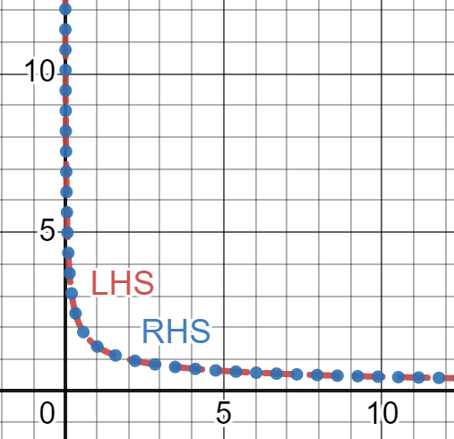
This plot appears to show us that the functions $z_{1}^{'}\left( t \right)$ and $4/z_{1}\left( t \right)$ are equal. Note: we have not graphed the function $z_{1}\left( t \right)$. The plots do not represent the solution function but rather the LHS and RHS functions. Note: this figure could be misleading. For instance, two functions could be very close, but not exactly equal to each other, but their graphs might appear indistinguishable. For the purposes of this course, however, we’ll assume that our figures are trustworthy.

Because LHS = RHS the function $z_{1}\left( t \right) = 2\sqrt{2t}$ is a solution to $z^{'} = \frac{4}{z}$ .

3.1.0.3 Example #3

Determine whether or not $u_{1}\left( t \right) = e^{- t}$ is a solution to this ODE: $u^{'} = u.$

$$\begin{aligned} &\text{LHS:}\quad u_{1}^{'} = \frac{d}{dt}\left[ e^{- t} \right] = - e^{- t}.\\ &\text{RHS:}\quad u_{1} = e^{- t}. \end{aligned}$$

Algebraically, we can see that $LHS \neq RHS$, so we know that $u_1(t)$ is not a solution to $u'=u$. If we insist on plotting the two, we get the figure below.

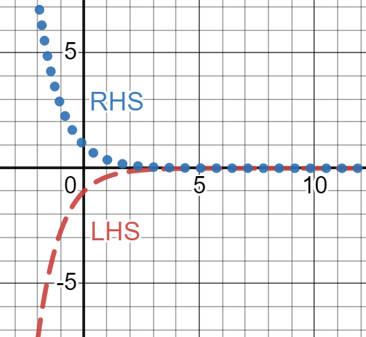
This figure also shows us that LHS $\neq$ RHS so the function $u_{1}\left( t \right) = e^{- t}$ is not a solution to $u' = u$ .

3.1.0.4 Example #4

Determine whether or not $w_{1}\left( t \right) = e^{t}\left( 2 + \sin\left( t \right) \right)$ is a solution to this ODE: $w^{'} = w + e^{t}\cos\left( t \right)$.

$$\begin{aligned} &\text{LHS:}\quad w_{1}' = \frac{d}{dt}\left[ e^{t}\left( 2 + \sin(t) \right)\right] = e^{t}\frac{d}{dt}\left[ 2 + \sin(t) \right] + \left( 2 + \sin(t) \right)\frac{d}{dt}\left[ e^{t} \right]\\ &\quad\quad\quad\quad\,\, = e^{t}\cos(t) + e^{t}\left( 2 + \sin(t) \right).\\ &\text{RHS:}\quad w_{1} + e^{t}\cos\left( t \right) = e^{t}\left( 2 + \sin\left( t \right) \right) + e^{t}\cos\left( t \right). \end{aligned}$$

Algebraically, we can see that LHS=RHS. If we plot the two, we get the figure below.

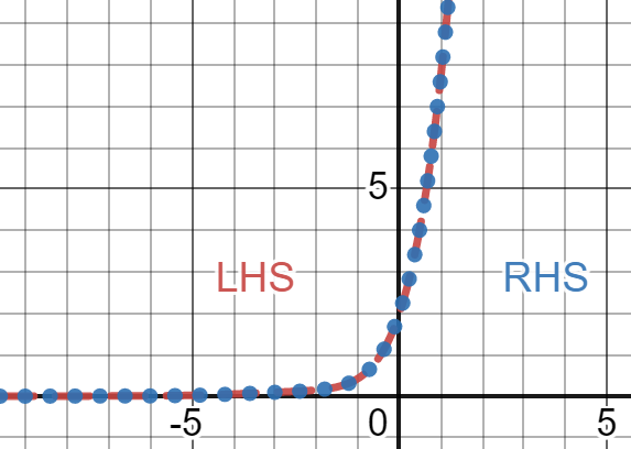
Since LHS = RHS, the function $w_{1}\left( t \right) = e^{t}\left( 2 + \sin\left( t \right) \right)$ is a solution to $w^{'} = w + e^{t}\cos\left( t \right)$ .

3.1.0.5 Example #5

Consider the differential equation $$y'=4y.$$ For what value of the parameter $D$ is $y_1=e^{Dt}$ a solution of the differential equation?

We proceed as in the problems above.

$$\begin{aligned} &\text{LHS:}\quad y_1'=De^{Dt}.\\ &\text{RHS:}\quad 4y_1=4e^{Dt}. \end{aligned}$$

In order to solve the differential equation, we need to have LHS=RHS, or $$De^{Dt}=4e^{Dt}.$$ We can see that the only way to satisfy this equation is by choosing $D=4$.

Indeed, $y_1=e^{4t}$ is a solution to the differential equation.

3.1.1 Order of Ordinary Differential Equations

There are many ways to classify ordinary differential equations. One very common one is called the order of the differential equation. The order of the differential equation is the order of the highest derivative of the unknown function in the ODE.

For example, the differential equation $$y'=3y$$ is first order, because the highest derivative on $y$ is a first derivative.

The differential equation $$y''+3y'+2y=0$$ is a second order differential equation, because the highest derivative on $y$ is a second derivative.

The differential equation $$y''+(y')^3=\cos(t)$$ is a second order differential equation.

In this class, we’ll stick to solving only first order differential equations, and systems of first order differential equations. However, it is important to be aware that there are many other types of equations besides those studied in this class.

3.2 Exercises

Determine whether or not each function is a solution to the given ODE. If a function is NOT a solution, plot the LHS function and the RHS function on the same set of axes. Comment on the difference between the two plots.

No.	ODE	Function 1	Function 2
1)	$y^{'} = y + e^{t}$	$y_1(t) = te^{t}$	$y_2(t) = 2e^{t}$
2)	$u^{'} = u$	$u_1(t) = 5e^{t}$	$u_2(t) = -3e^{t}$
3)	$z^{'} = -2z$	$z_1(t) = -2e^{t}$	$z_2(t) = -2e^{-2t}$
4)	$x^{'} = x - t$	$x_1(t) = e^{t} + t$	$x_2(t) = e^{t} + t + 1$
5)	$w^{'} = w^{2}$	$w_1(t) = \frac{1}{3-t}$	$w_2(t) = \frac{t^{3}}{3}$
6)	$y^{'} = \sqrt{y}$	$y_1(t) = \frac{t^{2}}{4}$	$y_2(t) = \frac{t^{4}}{4}$
7)	$z^{'} = 4(t^{3} - t)$	$z_1(t) = t^{4} - 2t^{2} + 1$	$z_2(t) = t^{4} - 2t^{2}$
8)	$x^{'} = 3x$	$x_1(t) = e^{3t} + 1$	$x_2(t) = e^{3t}$
9)	$w^{'} = \sqrt{t}$	$w_1(t) = \frac{2}{3}t^{3/2} + 1$	$w_2(t) = \frac{2}{3}t^{3/2}$
10)	$u^{'} = e^{2t}$	$u_1(t) = e^{2t}$	$u_2(t) = \frac{1}{2}e^{2t}$
11)	$y^{'} = \frac{t}{y}$	$y_1(t) = t$	$y_2(t) = -t$
12)	$u^{'} = u + 1$	$u_1(t) = 3e^{t} - 1$	$u_2(t) = 3e^{t} + 1$
13)	$z^{'} = \frac{1}{2z}$	$z_1(t) = \sqrt{7+t}$	$z_2(t) = \sqrt{7-t}$
14)	$x^{'} = \frac{x}{t}$	$x_1(t) = 3t$	$x_2(t) = t + 3$
15)	$w^{'} = \cos(t)w$	$w_1(t) = \sin(t)e^{t}$	$w_2(t) = e^{\sin(t)}$
16)	$z^{'} = 0$	$z_1(t) = t + 2$	$z_2(t) = 2$