Chapter 11 因子資料處理

因子物件 (factor) 為處理 類別資料 (categorical data), 提供的一種有效的方法. 類別變數 將變數值分成互斥的類別水準, 在類別變數定義中的特定幾種類別水準是否有大小差距, 又可分類成 名目變數 (nominal variable) 與 有序變數 (ordinal variable), 或稱 名目尺度 與 順序尺度.

在 {R} 中特別使用 因子 (factor) 來表示. 因子是一種特殊的文字向量, 文字向量中的每一個元素, 取一個離散值, 因子物件有一個特殊屬性, 稱為 層次, 水平, 水準 或 類別水準 (levels), 表示這組所有可能的離散值. 因子常常是用文字或字串輸入, 有時會使用數值或整數代表, 一但變數設定為因素或因子向量, {R} 在列印或輸出時, 並不會加上雙引號 ", 且數值或有大小順序的文字, {R} 在統計分析上都必須特別處理.

在 {R} 中若要設定因子, 可以簡單地用函式 factor() 產生無序因子物件.
tidyverse 套件系統提供 forcats 套件, 主要用來處理因子變數與類別資料.

11.1 forcats 套件: 基本函式

forcats 套件的基本函式包含

• fct_count(f, sort = FALSE, prop = FALSE): 計算類別水準數目.
• fct_unique(f): 呈現專一類別水準名稱.
• fct_c(f1, f2): 合併不同類別水準的 2 個因子物件.

library(dplyr)
library(ggplot2)
library(forcats)
library(kableExtra)
## Warning: package 'kableExtra' was built under R version 4.0.3
set.seed(100)
letters[1:5]
## [1] "a" "b" "c" "d" "e"
f <- factor(sample(letters[1:5])[rpois(100, 5)])
table(f)
## f
##  a  b  c  d  e 
## 21  2  3 21 15
fct_count(f)
## # A tibble: 6 x 2
##   f         n
##   <fct> <int>
## 1 a        21
## 2 b         2
## 3 c         3
## 4 d        21
## 5 e        15
## 6 <NA>     38
fct_count(f, sort = TRUE)
## # A tibble: 6 x 2
##   f         n
##   <fct> <int>
## 1 <NA>     38
## 2 a        21
## 3 d        21
## 4 e        15
## 5 c         3
## 6 b         2
fct_count(f, sort = TRUE, prop = TRUE)
## # A tibble: 6 x 3
##   f         n     p
##   <fct> <int> <dbl>
## 1 <NA>     38  0.38
## 2 a        21  0.21
## 3 d        21  0.21
## 4 e        15  0.15
## 5 c         3  0.03
## 6 b         2  0.02
##
f1 <- factor(letters[1:3])
f2 <- factor(letters[c(1, 2, 23)])
f1
## [1] a b c
## Levels: a b c
f2
## [1] a b w
## Levels: a b w
fct_c(f1, f2)
## [1] a b c a b w
## Levels: a b c w

11.2 移除或增加部分類別水準

資料分析中常因抽樣 0 值, 而必須特別處理, 例如必須移除部分類別水準或是必須增加因子變數中的類別水準. 下列函式可以執行這些功能.

fct_drop(f, only) # R baes  base::droplevels()
fct_expand(f, ...)
fct_explicit_na(f, na_level = "(Missing)")

函式 fct_drop() 可以移除部分類別水準, 函式 fct_expand() 可以增加因子變數中的類別水準. 函式 fct_explicit_na 可以明確設性缺失值為 1 項類別水準.

f <- factor(c("F", "M"), levels = c("F", "M", "Other"))
f
## [1] F M
## Levels: F M Other
fct_drop(f)
## [1] F M
## Levels: F M
# Set only to restrict which levels to drop
fct_drop(f, only = "F")
## [1] F M
## Levels: F M Other
fct_drop(f, only = "Other")
## [1] F M
## Levels: F M
## 
fct_expand(f, "B", "T")
## [1] F M
## Levels: F M Other B T
##
f <- factor(c("F", "M", "M", "F", "F", "B", "T", NA, NA))
f
## [1] F    M    M    F    F    B    T    <NA> <NA>
## Levels: B F M T
fct_explicit_na(f)
## [1] F         M         M         F         F         B         T         (Missing)
## [9] (Missing)
## Levels: B F M T (Missing)
fct_explicit_na(f, na_level = "Other")
## [1] F     M     M     F     F     B     T     Other Other
## Levels: B F M T Other

11.3 改變類別水準函式

因子變數中的類別水準的名稱呈現, 常常視需求而更改, 例如, H 改成 High, F 改成 female 等等. 函式 fct_recode() 可以改變的名稱呈現.

x <- factor(c("apple", "bear", "banana", "dear"))
x
## [1] apple  bear   banana dear  
## Levels: apple banana bear dear
fct_recode(x, fruit = "apple", fruit = "banana")
## [1] fruit bear  fruit dear 
## Levels: fruit bear dear
# If you name the level NULL it will be removed
fct_recode(x, NULL = "apple", fruit = "banana")
## [1] <NA>  bear  fruit dear 
## Levels: fruit bear dear
# When passing a named vector to rename levels use !!! to splice
x <- factor(c("apple", "bear", "banana", "dear"))
levels <- c(fruit = "apple", fruit = "banana")
fct_recode(x, !!!levels)
## [1] fruit bear  fruit dear 
## Levels: fruit bear dear
##
x <- factor(c("F", "M", "M", "F", "F", "B", "T"))
x
## [1] F M M F F B T
## Levels: B F M T
fct_recode(x, Male = "M", Female = "F", Other = "B", Other = "T")
## [1] Female Male   Male   Female Female Other  Other 
## Levels: Other Female Male

函式 fct_collapse() 可以改變的名稱呈現, 將不同類別水準合併且更名.

##
x <- factor(c("F", "M", "M", "F", "F", "B", "T"))
x
## [1] F M M F F B T
## Levels: B F M T
fct_collapse(x, Biological = c("M", "F"),
             Other = "B", Other = "T")
## [1] Biological Biological Biological Biological Biological Other      Other     
## Levels: Other Biological

函式 fct_other() 可將部分類別水準合併或移除.

fct_other(f, keep, drop, other_level = "Other")` 

其中引數 keep, drop 保留或移除部分原有類別水準, 將其餘類別水準合併成 other_level.

x <- factor(rep(LETTERS[1:4], times = 3))
x
##  [1] A B C D A B C D A B C D
## Levels: A B C D
fct_other(x, keep = c("A", "B"))
##  [1] A     B     Other Other A     B     Other Other A     B     Other Other
## Levels: A B Other
fct_other(x, drop = c("A", "B"), other_level = "change")
##  [1] change change C      D      change change C      D      change change C      D     
## Levels: C D change

11.4 改變或合併類別水準函式 fct_lump()

因子變數中的類別水準常常因頻率過低影響分析與推論, 常常常須要合併類別水準. 系列函式 fct_lump() 可將部分類別水準合併.

• fct_lump_min(): 合併類別水準頻率計數低於設定的最小值.
  
• `fct_lump_prop(): 合併類別水準相對頻率低於設定的最小值
  
• fct_lump_n(): 合併類別水準最多 n 種主要類別.
• fct_lump_lowfreq(): 合併類別水準, 且確保 other 類別的頻率仍是最低. 函式使用程式語言結構為

fct_lump(f, n, prop, w = NULL, other_level = "Other",
         ties.method = c("min", "average", "first", "last", "random", "max"))
fct_lump_min(f, min, w = NULL, other_level = "Other")
fct_lump_prop(f, prop, w = NULL, other_level = "Other")
fct_lump_n(f, n, w = NULL, other_level = "Other",
  ties.method = c("min", "average", "first", "last", "random", "max"))
fct_lump_lowfreq(f, other_level = "Other")

其中引數 f 為因子向量, n 設定最多 n 種主要類別, prop 設定正值百分率, 合併小於 prop 的類別, 設定負值百分率, 合併大於 prop 的類別. w 設定權重. other_level 設定合併後的類別名稱. ties.method 處理相同排序方式. min 保留至少出現 min 次類別.

x <- factor(rep(LETTERS[1:9], times = c(40, 10, 5, 27, 1, 1, 1, 1, 1)))
x %>% table()
## .
##  A  B  C  D  E  F  G  H  I 
## 40 10  5 27  1  1  1  1  1
x %>% fct_lump_n(3) %>% table()
## .
##     A     B     D Other 
##    40    10    27    10
x %>% fct_lump_prop(0.10) %>% table()
## .
##     A     B     D Other 
##    40    10    27    10
x %>% fct_lump_min(5) %>% table()
## .
##     A     B     C     D Other 
##    40    10     5    27     5
x %>% fct_lump_lowfreq() %>% table()
## .
##     A     D Other 
##    40    27    20
##
set.seed(123)
x <- factor(letters[rpois(50, 5)])
x
##  [1] d g d h i b e h e e i e f e b h c b d i h f f k f f e e d c i h f g a e f c d c c d
## [43] d d c c c e d g
## Levels: a b c d e f g h i k
table(x)
## x
## a b c d e f g h i k 
## 1 3 8 9 9 7 3 5 4 1
table(fct_lump_lowfreq(x))
## 
##     b     c     d     e     f     g     h     i Other 
##     3     8     9     9     7     3     5     4     2
## Use positive values to collapse the rarest
fct_lump_n(x, n = 3)
##  [1] d     Other d     Other Other Other e     Other e     e     Other e     Other e    
## [15] Other Other c     Other d     Other Other Other Other Other Other Other e     e    
## [29] d     c     Other Other Other Other Other e     Other c     d     c     c     d    
## [43] d     d     c     c     c     e     d     Other
## Levels: c d e Other
fct_lump_prop(x, prop = 0.1)
##  [1] d     Other d     Other Other Other e     Other e     e     Other e     f     e    
## [15] Other Other c     Other d     Other Other f     f     Other f     f     e     e    
## [29] d     c     Other Other f     Other Other e     f     c     d     c     c     d    
## [43] d     d     c     c     c     e     d     Other
## Levels: c d e f Other
## Use negative values to collapse the most common
fct_lump_n(x, n = -3)
##  [1] Other g     Other Other Other b     Other Other Other Other Other Other Other Other
## [15] b     Other Other b     Other Other Other Other Other k     Other Other Other Other
## [29] Other Other Other Other Other g     a     Other Other Other Other Other Other Other
## [43] Other Other Other Other Other Other Other g    
## Levels: a b g k Other
fct_lump_prop(x, prop = -0.1)
##  [1] Other g     Other h     i     b     Other h     Other Other i     Other Other Other
## [15] b     h     Other b     Other i     h     Other Other k     Other Other Other Other
## [29] Other Other i     h     Other g     a     Other Other Other Other Other Other Other
## [43] Other Other Other Other Other Other Other g    
## Levels: a b g h i k Other
## Use weighted frequencies
w <- c(rep(2, 25), rep(1, 25))
fct_lump_n(x, n = 5, w = w)
##  [1] d     Other d     h     Other Other e     h     e     e     Other e     f     e    
## [15] Other h     c     Other d     Other h     f     f     Other f     f     e     e    
## [29] d     c     Other h     f     Other Other e     f     c     d     c     c     d    
## [43] d     d     c     c     c     e     d     Other
## Levels: c d e f h Other
fct_lump_n(x, n = 6)
##  [1] d     Other d     h     i     Other e     h     e     e     i     e     f     e    
## [15] Other h     c     Other d     i     h     f     f     Other f     f     e     e    
## [29] d     c     i     h     f     Other Other e     f     c     d     c     c     d    
## [43] d     d     c     c     c     e     d     Other
## Levels: c d e f h i Other
fct_lump_n(x, n = 6, ties.method = "max")
##  [1] d     Other d     h     i     Other e     h     e     e     i     e     f     e    
## [15] Other h     c     Other d     i     h     f     f     Other f     f     e     e    
## [29] d     c     i     h     f     Other Other e     f     c     d     c     c     d    
## [43] d     d     c     c     c     e     d     Other
## Levels: c d e f h i Other
## Use fct_lump_min() to lump together all levels with fewer than `n` values
table(fct_lump_min(x, min = 10))
## 
## Other 
##    50

以第 5 章中 退伍軍人肺癌臨床試驗 資料 (survVATrial.csv) 為例, 細胞型態 cellcode 有 4 種類別. 將類別水準合併成 2 種主要類別, 其餘類別合併.

dd <- read.table("./Data/survVATrial.csv",
                 header = TRUE,
                 sep = ",",
                 quote = "\"'",
                 dec = ".",
                 row.names = NULL,
                 # col.names,
                 as.is = TRUE,
                 # as.is = !stringsAsFactors,
                 na.strings = c(".", "NA"))
head(dd)
##   treat cellcode time censor diagtime kps age prior
## 1     0        1   72      1       60   7  69     0
## 2     0        1  411      1       70   5  64    10
## 3     0        1  228      1       60   3  38     0
## 4     0        1  126      1       60   9  63    10
## 5     0        1  118      1       70  11  65    10
## 6     0        1   10      1       20   5  49     0
str(dd)
## 'data.frame':    137 obs. of  8 variables:
##  $ treat   : int  0 0 0 0 0 0 0 0 0 0 ...
##  $ cellcode: int  1 1 1 1 1 1 1 1 1 1 ...
##  $ time    : int  72 411 228 126 118 10 82 110 314 100 ...
##  $ censor  : int  1 1 1 1 1 1 1 1 1 0 ...
##  $ diagtime: int  60 70 60 60 70 20 40 80 50 70 ...
##  $ kps     : int  7 5 3 9 11 5 10 29 18 6 ...
##  $ age     : int  69 64 38 63 65 49 69 68 43 70 ...
##  $ prior   : int  0 10 0 10 10 0 10 0 0 0 ...
dd$treat <- factor(dd$treat, labels = c("placebo", "test"))
dd$cellcode <- factor(dd$cellcode, 
                      labels = c("squamous", "small", "adeno", "large"))
dd$censor <- factor(dd$censor, labels = c("survival", "dead"))
dd$prior <- factor(dd$prior, labels = c("no", "yes"))
head(dd)
##     treat cellcode time censor diagtime kps age prior
## 1 placebo squamous   72   dead       60   7  69    no
## 2 placebo squamous  411   dead       70   5  64   yes
## 3 placebo squamous  228   dead       60   3  38    no
## 4 placebo squamous  126   dead       60   9  63   yes
## 5 placebo squamous  118   dead       70  11  65   yes
## 6 placebo squamous   10   dead       20   5  49    no
str(dd)
## 'data.frame':    137 obs. of  8 variables:
##  $ treat   : Factor w/ 2 levels "placebo","test": 1 1 1 1 1 1 1 1 1 1 ...
##  $ cellcode: Factor w/ 4 levels "squamous","small",..: 1 1 1 1 1 1 1 1 1 1 ...
##  $ time    : int  72 411 228 126 118 10 82 110 314 100 ...
##  $ censor  : Factor w/ 2 levels "survival","dead": 2 2 2 2 2 2 2 2 2 1 ...
##  $ diagtime: int  60 70 60 60 70 20 40 80 50 70 ...
##  $ kps     : int  7 5 3 9 11 5 10 29 18 6 ...
##  $ age     : int  69 64 38 63 65 49 69 68 43 70 ...
##  $ prior   : Factor w/ 2 levels "no","yes": 1 2 1 2 2 1 2 1 1 1 ...
##
dd %>% select(cellcode) %>% table()
## .
## squamous    small    adeno    large 
##       35       48       27       27
dd %>% select(cellcode) %>% 
  mutate(cellcode = fct_lump(cellcode, n = 1)) %>% 
  table()
## .
## small Other 
##    48    89

11.5 類別水準的頻率排序函式 fct_infreq()

函式系列 fct_infreq() 可將類別水準的頻率排序記錄.

• fct_inorder(): 依照類別水準出現的次序排序.
  
• fct_infreq(): 依照類別水準的頻率排序 (由多到少).
  
• fct_inseq(): 依照類別水準的儲存數值排序.

f <- factor(c("b", "b", "a", "c", "c", "c"))
f
## [1] b b a c c c
## Levels: a b c
fct_inorder(f)
## [1] b b a c c c
## Levels: b a c
fct_infreq(f)
## [1] b b a c c c
## Levels: c b a
##
f <- factor(1:3, levels = c("3", "2", "1"))
f
## [1] 1 2 3
## Levels: 3 2 1
#> Levels: 3 2 1
fct_inseq(f)
## [1] 1 2 3
## Levels: 1 2 3

以第 5 章中 退伍軍人肺癌臨床試驗 資料 (survVATrial.csv) 為例, 細胞型態 cellcode 有 4 種類別.

dd %>% select(cellcode) %>% table()
## .
## squamous    small    adeno    large 
##       35       48       27       27
## fct_inorder()
dd %>% select(cellcode) %>% 
  mutate(cellcode = fct_inorder(cellcode)) %>% 
  table()
## .
## squamous    small    adeno    large 
##       35       48       27       27
## fct_infreq()
dd %>% select(cellcode) %>% 
  mutate(cellcode = fct_infreq(cellcode)) %>% 
  table()
## .
##    small squamous    adeno    large 
##       48       35       27       27
## fct_inseq()
dd %>% select(cellcode) %>% 
  mutate(cellcode = fct_inseq(factor(as.numeric(cellcode)))) %>% table()
## .
##  1  2  3  4 
## 35 48 27 27

以第 5 章中 退伍軍人肺癌臨床試驗 資料 (survVATrial.csv) 為例, 細胞型態 cellcode 有 4 種類別. 首先繪製長條圖.

## barplot
ggplot(dd, aes(x = cellcode)) + 
  geom_bar() + 
  coord_flip()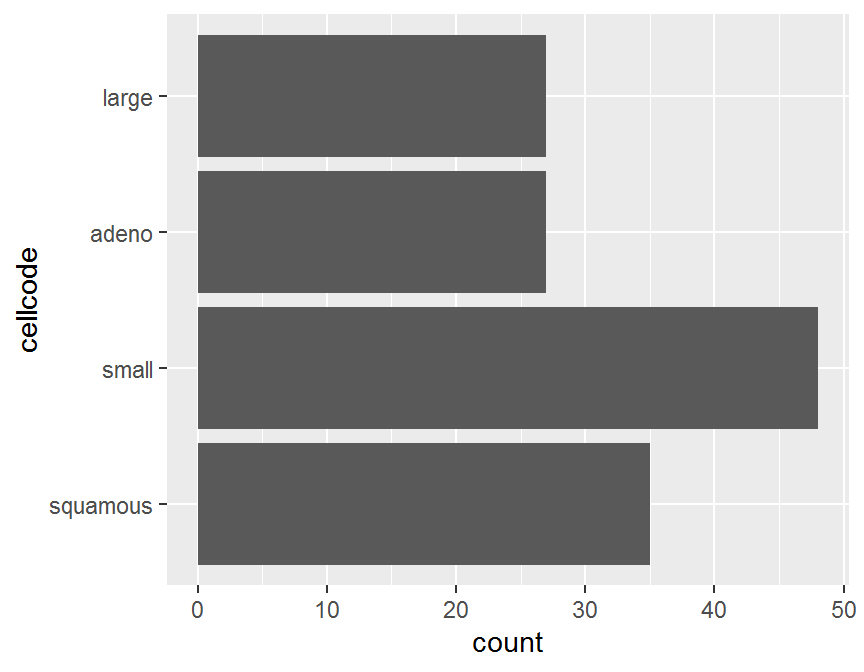

圖中的類別出現並非照類別水準的頻率順序, 函式 fct_infreq() 可將類別水準的頻率排序記錄.

ggplot(dd, aes(x = fct_infreq(cellcode))) + 
  geom_bar() + 
  coord_flip()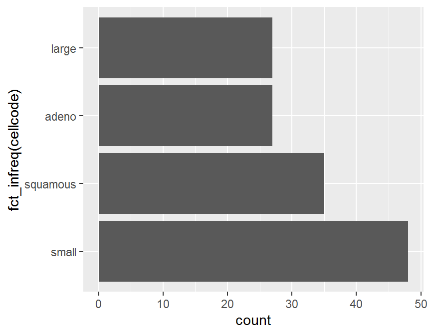

11.6 依照其他變數將類別重新排序函式 fct_reorder()

因子變數中的類別水準常常因其他變數而須將類別重新排序.

• fct_rev(f): 將反轉原有類別出現的排列順序.
• fct_shuffle(f, n = 1L): 將原有類別出現的排列順序隨機變更.
• fct_reorder(.f, .x, .fun = median, ..., .desc = FALSE)
• fct_reorder2(.f, .x, .y, .fun = last2, ..., .desc = TRUE)
• first2(.x, .y)
• last2(.x, .y)

fct_reorder() 將因子 f 類別出現的排列順序依照其他變數更動, fct_reorder2() 保留因子 f 原有類別出現的排列順序. 當 y 變數依照 x 變數排序, 函式 first2(.x, .y) 與 last2(.x, .y)
可尋找 y 變數的最前與最後的 2 個數值. 其中引數

• .f: 為主要因子變數.
• .x, .y: 為其他變數.
• .fun: 為摘要函式.
• .desc = FALSE 由小到大排序.

f <- factor(c("a", "b", "c"))
fct_rev(f)
## [1] a b c
## Levels: c b a
fct_shuffle(f)
## [1] a b c
## Levels: a c b
fct_shuffle(f)
## [1] a b c
## Levels: c b a
##
df <- tibble::tribble(
  ~color,     ~a, ~b,
  "blue",      1,  2,
  "green",     6,  2,
  "purple",    3,  3,
  "red",       2,  3,
  "yellow",    5,  1
)
df$color <- factor(df$color)
##
fct_reorder(df$color, df$a, min)
## [1] blue   green  purple red    yellow
## Levels: blue red purple yellow green
fct_reorder2(df$color, df$a, df$b)
## [1] blue   green  purple red    yellow
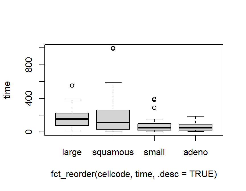
## Levels: purple red blue green yellow

以第 5 章中 退伍軍人肺癌臨床試驗 資料 (survVATrial.csv) 為例, 細胞型態 cellcode 有 4 種類別.

boxplot(time ~ cellcode, data = dd)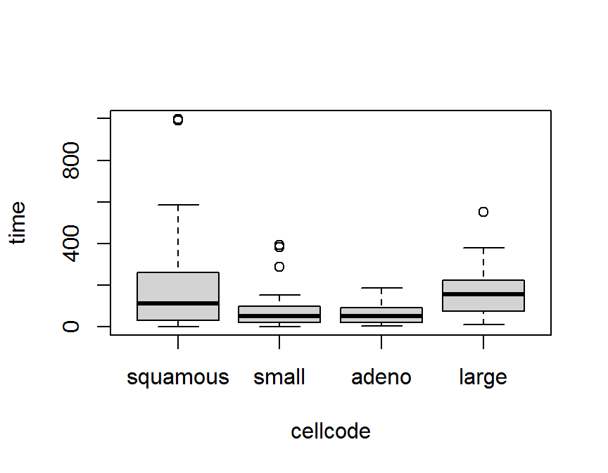

boxplot(time ~ fct_reorder(cellcode, time), data = dd)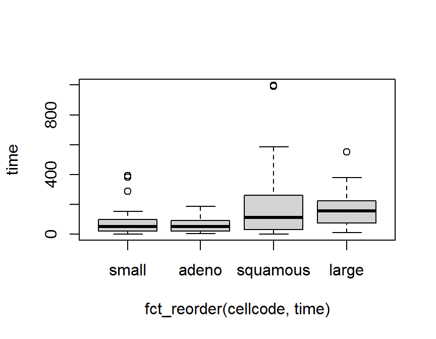

boxplot(time ~ fct_reorder(cellcode, time, .desc = TRUE), data = dd)