Chapter 8 資料基本處理

tidyverse 套件系統 包含許多不同套件, 提供資料科學一些實用的函式. 包含

• tidyverse 核心
  • ggplot2 視覺化分析.
  • purrr 執行迴圈.
  • tibble 增強資料框架.
  • dplyr 資料處裡.
  • tidyr 精簡資料,
  • stringr 字串整理.
  • readr 資料輸入.
  • forcats 處理類別變數 (factors).

tidyverse 套件系統的其他關聯套件包含

• 資料輸入 import
  • readxl 輸入 excel 關聯檔案.
    
  • haven 輸入 SPSS, Stata 與 SAS 關聯檔案.
  • jsonlite 輸入 JSON 關聯檔案.
  • xml2 輸入 XML 關聯檔案.
  • httr 輸入 web APIs 關聯檔案.
  • rvest 輸入 web scraping 關聯檔案.
• DBI 輸入 關聯資料庫, 協同套件有 RSQLite, RPostgres 或 odbc.
• 資料處理 tidy/wrangle
  • stringr 處理字串.
  • lubridate 處理日期與時間.
  • forcats 處理類別變數 (factors).
  • hms 處理日期與時間.
  • blob 處理二元資料儲存檔案.
• 程式寫作 program
  • rlang 提供寫作核心語言與 tidyverse.
  • magrittr 提供資料流動通道 %>%.
  • glue 提供字串合併.
• 建模 model
  • broom 處理建模結果.
  • modelr 偕同執行建模族.

8.1 資料輸入套件 readr

tidyverse 套件系統中的 readr 套件提供一些方便資料輸入的函式. 包含 read_csv() 輸入 .csv 資料檔, read_excel 輸入 excel 資料檔, read_delim() 輸入不同分隔符號資料檔. 其中引數如下 (help(read_delim)).

read_delim(
  file,
  delim,
  quote = "\"",
  escape_backslash = FALSE,
  escape_double = TRUE,
  col_names = TRUE,
  col_types = NULL,
  locale = default_locale(),
  na = c("", "NA"),
  quoted_na = TRUE,
  comment = "",
  trim_ws = FALSE,
  skip = 0,
  n_max = Inf,
  guess_max = min(1000, n_max),
  progress = show_progress(),
  skip_empty_rows = TRUE
)

• file = 路徑與檔名
• delim = 分隔符號
• quote = 視同分隔符號 (資料的文字變數值常放在雙引號中)
• escape_backslash = 預設 FALSE, 是否有逃脫符號
• escape_double = 預設TRUE, 是否用引號符號作為逃脫符號
• col_names = 設定變數名 (T 或 F)
• col_types = 設定變數的類型
• na = 設定 NA 符號
• comment = 設定注釋符號, 在注釋符號之後的文字不會被讀入
• trim_ws = 去除變數值得空白
• skip = 要跳過幾行 (row) 才開始讀入資料
• n_max = 最大輸入行數

糖尿病與人工關節術後感染臨床試驗 (糖尿病與人工全膝關節置換手術研究)

退化性膝關節炎是人類關節疾病中最常見的一種, 主要病變的地方是膝關節的的關節軟骨受到傷害與磨損, 造成關節腔變窄以及產生骨刺, 變化與年紀有高度相關. 年長者患有嚴重退化性膝關節炎, 常須進行人工全膝關節置換手術 (TKR), 但是若是術後感染, 則有可能照造成截肢或因敗血症而死亡, 且糖尿病 (DM) 患者是此全膝關節置換手術後感染的高危險群. 因此一位骨科醫師進行一預防性臨床試驗, 對患有嚴重退化性膝關節炎的糖尿病患者, 隨機分配 2 組, 一組在全膝關節置換手術中, 使用的骨水泥內, 加入預防性抗生素藥劑, 另一組為對照組. 研究的主要目的是探討全膝關節置換手術中, 在骨水泥內加入預防性抗生素藥劑, 是否可以預防術後感染. 另外一個研究目的是在骨水泥內加入預防性抗生素藥劑, 研究共收集了 78 位病患的資料, 變數名稱列在表 1. 資料檔案為 DMTKRcsv.csv, DMTKAInfMo.csv, DMTKRtabsep.txt 與 DMTKRblanksep.txt.

變數	說明
NO	病患辨識碼
AGE	年紀歲數 (單位: 年) (age)
SEX	性別: 0 = F = 女 (female), 1 = M = 男 (Male).
DM	糖尿病形態: 0 = Type II (NIDDM); 1 = Type I (IDDM)
DMYR	手術前糖尿病病史 (單位: 年)
PREAC	手術前空腹血糖 (mg/dL)
PREPC	手術前飯後血糖 (mg/dL)
POSTAC	手術後空腹血糖 (mg/dL)
POSTPC	手術後飯後血糖 (mg/dL)
MEDICATION	糖尿病治療方式:
	0 = 口服降血糖藥劑; 1 = 胰島素注射; 2 = 飲食控制
SIDE	患側: 0 = 左側; 1 = 右側
PREKS	手術前膝功能分數
POSTKS	手術後膝功能分數
ABS	骨水泥是否加抗生素 1 = Yes; 0 = No
INFECT	術後感染: 0 = No; 1 = Yes, 發現術後感染
INFMO	發現術後感染的時間 (單位: 月)
MISC	註記

Table 1. 糖尿病與人工關節術後感染臨床試驗: 變數說明

# .csv
library(tidyverse)
## Warning: package 'tibble' was built under R version 4.0.3
## Warning: package 'readr' was built under R version 4.0.3
library(readr)
dd <- readr::read_csv("./Data/DMTKAInfMo.csv")
print(dd, n = 5, width = Inf)
## # A tibble: 78 x 16
##      No   age   sex    DM  DMyr preAC prePC postAC postPC medication  SIDE PREKS POSTKS
##   <dbl> <dbl> <dbl> <dbl> <dbl> <dbl> <dbl>  <dbl>  <dbl>      <dbl> <dbl> <dbl>  <dbl>
## 1     1    67     0     0    10   120   160    140    180          0     0    56     92
## 2     2    67     0     0    11   100   150    150    220          0     1    62     62
## 3     3    72     1     0     4   150   200    120    150          2     0    60     94
## 4     4    82     1     0     8   150   200    160    250          0     1    47     90
## 5     5    73     1     0     3    85   110    140    200          0     0    44     88
##     ABS INFECT INFMO
##   <dbl>  <dbl> <dbl>
## 1     1      0     0
## 2     0      1     2
## 3     1      0     0
## 4     1      0     0
## 5     0      0     0
## # ... with 73 more rows
# .xls
library(readxl)
dd <- readxl::read_excel("C:/RData/DMTKAInfMo.xls")
print(dd, n = 5, width = Inf)
## # A tibble: 78 x 16
##      No   age   sex    DM  DMyr preAC prePC postAC postPC medication  SIDE PREKS POSTKS
##   <dbl> <dbl> <dbl> <dbl> <dbl> <dbl> <dbl>  <dbl>  <dbl>      <dbl> <dbl> <dbl>  <dbl>
## 1     1    67     0     0    10   120   160    140    180          0     0    56     92
## 2     2    67     0     0    11   100   150    150    220          0     1    62     62
## 3     3    72     1     0     4   150   200    120    150          2     0    60     94
## 4     4    82     1     0     8   150   200    160    250          0     1    47     90
## 5     5    73     1     0     3    85   110    140    200          0     0    44     88
##     ABS INFECT I0FECTMO
##   <dbl>  <dbl>    <dbl>
## 1     1      0        0
## 2     0      1        2
## 3     1      0        0
## 4     1      0        0
## 5     0      0        0
## # ... with 73 more rows

8.2 整潔資料 Tidy Data

統計計算可以進行分析的資料, 通常有一個的簡單的基本架構, 在 {R} 稱作 資料框架 (data frame). 資料框架是類似於在 SAS, STATA 等的 dataset 架構. 資料框架通常類似矩陣, 資料框架也類似矩形的 交叉列聯表 (cross table), 稱為 資料表 (** data table). 套件 tidverse 原始套件 tidy` 強調外部資料檔案必須符合 整潔資料** (tidy data) 方便操作. 整潔資料的基本要求特徵是 每個變數各自形成 1 欄 (縱行, row), 每個列 (橫列, row) 各自為一個觀測時間的測量. 例如, 每位個體只有觀測一次, 則每個列為一位個體的觀測值. 若每位個體有多次觀測時間點, 則一位個體一次觀測時間點的觀測值為一列, 一位個體或有多列的觀測值. 一個整潔資料的資料表包含以下重點.

• 一個檔案只用一張資料表
• 一張資料表 (EXCEL 的 sheet).
• 一個欄位 (縱行, Column) 只有一個變數, 同時有清楚的變數名.
• 若完整資料包含不同資料表, 則不同資料表要有索引 (inxex) 或指標變數 (id) 可進行關聯與串聯.

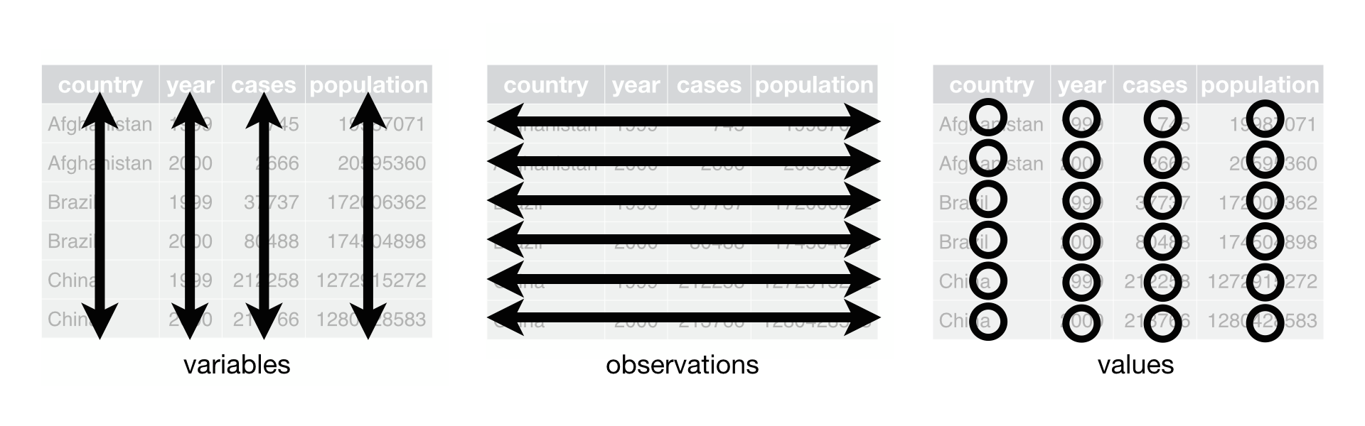
Tidy Data: R for Data Science, Figure 12.1

整潔資料 指引主要提供研究者在輸入資料檔案時能夠遵循. 例如, 一些者常將 EXCEL 一張 sheel 內混合著原始資料, 分析結果與圖形. 也經常將二個變數放在同一個欄位, 二個變數簡單以 / 分隔. 例如檔案 DMTKAORI.xls. 若資料檔案不是整潔資料, 則需浩費學多時間清理, 甚至必須重新輸入到資料檔案.

8.3 Tibble 與 Data Frame

tidyverse 系統中的 readr 套件輸入資料後, tidyverse 會儲存成 (tibble) 資料物件, 成為tbl_df, tbl 類型的資料物件, 主要是 tidyverse 系統會使用 tibble 套件進行操作. tibbles 資料物件與原有資料框架 data.frame 物件有相同的屬性外, 另外多了些讓 tidyverse 系統容易操作的屬性. 對初學者而言, 二者幾呼無任何差異. 若有 {R} base 函式無法操作 tibble 資料物件, 可使用 as.data.frame() 轉成 {R} base 的 data.frame 物件. 同樣, 若 tidyverse 系統函式無法操作的 data.frame 物件, 可用 ‵as_tibble()將data.frame物件 轉成tibbles` 資料物件. 以資料在檔案第 5 章的 survVATrial.csv 為例.

## data frame object
dd <- read.table("./Data/survVATrial.csv",
                 header = TRUE,
                 sep = ",",
                 quote = "\"'",
                 dec = ".",
                 row.names = NULL,
                 # col.names,
                 as.is = TRUE,
                 # as.is = !stringsAsFactors,
                 na.strings = c(".", "NA"))
class(dd)
## [1] "data.frame"
library(tibble)
dd <- as_tibble(dd)
class(dd)
## [1] "tbl_df"     "tbl"        "data.frame"

tibble 套件的 tibble() 函式的使用如同 {R} base data.frame(). tibble() 函式可以使用 {R} base 不准使用的變數名. tibble 物件與 data.frame 物件的主要差別有 2 種情境.

1. tibble 物件的顯示, print() 只用 10 rows, 變數 (columns) 只有納入符合視窗寬度的數目, 這對大數據檢視較為方便. 且顯示 str() 函式可呈現變數基本模式的類別. 可使用 n = k 顯示 \(k\) rows, width = Inf 顯示所有變數. 也可設定整區選項為 options(tibble.print_min = Inf), 顯示所有 rows, 以及 options(tibble.width = Inf) 顯示所有 columns.

2. {R} base 多數容許使用部分物件名 (變數名), 但 tibble 物件無法使用部分變數名. 可能會對資深程式寫作人員些許困擾.

8.4 資料流動管道運算指令 Pipe

tidyverse 系統中的 magrittr 套件提供一個非常實用的運算指令 %>% 稱為 pipe, 管線, 管道, 導管. 此運算符號, 可將函式與運算串聯, %>% 左側通常是資料物件, 資料框架, 矩陣, 向量等, %>% 右側通常是函式 fun_name(), 而 %>% 左側資料自動為函式 fun_name() 內的第一個引數. 在 Unix/Linux 系統的各種指令可以運用 pipe 的方式串連執行, magrittr 套件提供類似的思維, 且資料流動從 %>% 左測的資料送到 %>%右側的函式執行運算, 可讓程式寫作符合文字書寫由左到右的思考邏輯. 使用pipe` 並不會改變程式的執行順序, 主要目的在於讓程式更容易寫作與閱讀, 降低程式寫作的錯誤與負擔.

## short and clean 
log(mean(c(1:10)))
## [1] 1.705
## easily read 
x <- c(1:10)
x.mean <- mean(x)
log.mean <- log(x.mean)
log.mean
## [1] 1.705
## pipe %>%
library(magrittr)
c(1:10) %>% mean() %>% log()
## [1] 1.705

8.5 資料檢視函式 glimpse()

資料輸入到 {R} 後, 必須先檢視資料內容, 比對原始資料檔案是否正確讀入資料. 包含觀測值數目, 變數數目, 那些變數為辨識指標, 變數屬性, 那些變數為連續變數或類別變數, 類別變數屬性, 名目變數或是順序變數, 整理類別變數的類別水準名稱. 每個變數的缺失數目與頻率, 每個個體的缺失數目與頻率. 以資料在檔案第 5 章的 survVATrial.csv 為例.

dd = dd %>% as_tibble()
print(dd, n = 5, width = Inf)
## # A tibble: 137 x 8
##   treat cellcode  time censor diagtime   kps   age prior
##   <int>    <int> <int>  <int>    <int> <int> <int> <int>
## 1     0        1    72      1       60     7    69     0
## 2     0        1   411      1       70     5    64    10
## 3     0        1   228      1       60     3    38     0
## 4     0        1   126      1       60     9    63    10
## 5     0        1   118      1       70    11    65    10
## # ... with 132 more rows

可以看到資料有 137 位個體, 8 個變數. 其中time, diagtime, kps, age 為連續變數. treat, cellcode, censor, prior 等為類別變數, 但類別變數以數字輸入, 需先設定成為類別變數. 以資料在檔案第 5 章的 survVATrial.csv 為例.

dd$treat <- factor(dd$treat, labels = c("placebo", "test"))
dd$cellcode <- factor(dd$cellcode, 
                      labels = c("squamous", "small", "adeno", "large"))
dd$censor <- factor(dd$censor, labels = c("survival", "dead"))
dd$prior <- factor(dd$prior, labels = c("no", "yes"))
print(dd, n = 5, width = Inf)
## # A tibble: 137 x 8
##   treat   cellcode  time censor diagtime   kps   age prior
##   <fct>   <fct>    <int> <fct>     <int> <int> <int> <fct>
## 1 placebo squamous    72 dead         60     7    69 no   
## 2 placebo squamous   411 dead         70     5    64 yes  
## 3 placebo squamous   228 dead         60     3    38 no   
## 4 placebo squamous   126 dead         60     9    63 yes  
## 5 placebo squamous   118 dead         70    11    65 yes  
## # ... with 132 more rows

tidyverse 系統中的 tibble 套件提供一個檢視資料函式 `glimpse(), 類似 {R} base 的 str() 函式.

## R base
str(dd)
## tibble [137 x 8] (S3: tbl_df/tbl/data.frame)
##  $ treat   : Factor w/ 2 levels "placebo","test": 1 1 1 1 1 1 1 1 1 1 ...
##  $ cellcode: Factor w/ 4 levels "squamous","small",..: 1 1 1 1 1 1 1 1 1 1 ...
##  $ time    : int [1:137] 72 411 228 126 118 10 82 110 314 100 ...
##  $ censor  : Factor w/ 2 levels "survival","dead": 2 2 2 2 2 2 2 2 2 1 ...
##  $ diagtime: int [1:137] 60 70 60 60 70 20 40 80 50 70 ...
##  $ kps     : int [1:137] 7 5 3 9 11 5 10 29 18 6 ...
##  $ age     : int [1:137] 69 64 38 63 65 49 69 68 43 70 ...
##  $ prior   : Factor w/ 2 levels "no","yes": 1 2 1 2 2 1 2 1 1 1 ...
## glimpse()
glimpse(dd)
## Rows: 137
## Columns: 8
## $ treat    <fct> placebo, placebo, placebo, placebo, placebo, placebo, placebo, pla...
## $ cellcode <fct> squamous, squamous, squamous, squamous, squamous, squamous, squamo...
## $ time     <int> 72, 411, 228, 126, 118, 10, 82, 110, 314, 100, 42, 8, 144, 25, 11,...
## $ censor   <fct> dead, dead, dead, dead, dead, dead, dead, dead, dead, survival, de...
## $ diagtime <int> 60, 70, 60, 60, 70, 20, 40, 80, 50, 70, 60, 40, 30, 80, 70, 60, 60...
## $ kps      <int> 7, 5, 3, 9, 11, 5, 10, 29, 18, 6, 4, 58, 4, 9, 11, 3, 9, 2, 4, 4, ...
## $ age      <int> 69, 64, 38, 63, 65, 49, 69, 68, 43, 70, 81, 63, 63, 52, 48, 61, 42...
## $ prior    <fct> no, yes, no, yes, yes, no, yes, no, no, no, no, yes, no, yes, yes,...

8.6 資料處裡 dplyr 套件

tidyverse 系統中的資料處裡 dplyr 套件, 有一些資料資料處裡常用函式.

• %>% = pipe 指令
• rename() = 變數 (column) 重新命名
• filter() = 選擇個體或行位子集 (rows)
• arrange() = 依據變數值排序
• select() = 選擇變數 (variables) 或欄位子集 (columns)
• mutate() = 變數轉換
• sample_n() 與 sample_frac() = 隨機抽樣函式
• distinct() 與 n_distinct() = 選出明顯不同個體
• slice() = 利用橫列指標 (row index) 選出個體 (row)
• summarise() = 計算常見統計量
• group_by() = 資料分組操作

這些函式的第 1 個引數為資料物件, 後續只用為變數名 (不加雙引號), 可以合併使用 group_by() 函式與 %>% 指令.

8.6.1 選擇個體函式 filter()

資料常常需要依據納入與排除條件, 此時會依據變數值進行篩選. filter() 函式可協助選擇個體. 以資料在檔案第 5 章的 survVATrial.csv 為例, 選擇個體 treat 為 placebo, cellcode 為 large.

## filter()
dd.a <- dd %>% 
  filter(treat == 'placebo', cellcode == 'large')
dd.a
## # A tibble: 15 x 8
##    treat   cellcode  time censor   diagtime   kps   age prior
##    <fct>   <fct>    <int> <fct>       <int> <int> <int> <fct>
##  1 placebo large      177 dead           50    16    66 yes  
##  2 placebo large      162 dead           80     5    62 no   
##  3 placebo large      216 dead           50    15    52 no   
##  4 placebo large      553 dead           70     2    47 no   
##  5 placebo large      278 dead           60    12    63 no   
##  6 placebo large       12 dead           40    12    68 yes  
##  7 placebo large      260 dead           80     5    45 no   
##  8 placebo large      200 dead           80    12    41 yes  
##  9 placebo large      156 dead           70     2    66 no   
## 10 placebo large      182 survival       90     2    62 no   
## 11 placebo large      143 dead           90     8    60 no   
## 12 placebo large      105 dead           80    11    66 no   
## 13 placebo large      103 dead           80     5    38 no   
## 14 placebo large      250 dead           70     8    53 yes  
## 15 placebo large      100 dead           60    13    37 yes

選擇個體 treat 為試驗藥組, age 大於 50, kps 小於或等於 7

dd.b <- dd %>% 
  filter(treat == 'test', age > 50, kps <= 7)
dd.b
## # A tibble: 35 x 8
##    treat cellcode  time censor diagtime   kps   age prior
##    <fct> <fct>    <int> <fct>     <int> <int> <int> <fct>
##  1 test  squamous   112 dead         80     6    60 no   
##  2 test  squamous   242 dead         50     1    70 no   
##  3 test  squamous   111 dead         70     3    62 no   
##  4 test  squamous   587 dead         60     3    58 no   
##  5 test  squamous   389 dead         90     2    62 no   
##  6 test  squamous    33 dead         30     6    64 no   
##  7 test  squamous   467 dead         90     2    64 no   
##  8 test  squamous   283 dead         90     2    51 no   
##  9 test  small       25 dead         30     2    69 no   
## 10 test  small       21 dead         20     4    71 no   
## # ... with 25 more rows

8.6.2 依據變數值排序函式 arrange()

資料常常需要依據變數值排序, arrange() 函式內設依照變數在函式出現順序以及變數值由小到大排序. 若要變數值從由大到小排序, 可使用 desc() 函式. 例如, 以資料在檔案第 5 章的 survVATrial.csv 為例, 依照 age 由小到大排序, time 由大到小排序. 無論如何排序, 缺失值總是排在最後, 這須與 {R} base 的 order(), sort() 或 rank() 進行比較.

## arrange()
dd.s <- dd %>% 
  arrange(age, desc(time))
dd.s
## # A tibble: 137 x 8
##    treat   cellcode  time censor   diagtime   kps   age prior
##    <fct>   <fct>    <int> <fct>       <int> <int> <int> <fct>
##  1 placebo adeno       95 dead           80     4    34 no   
##  2 placebo small        4 dead           40     2    35 no   
##  3 test    squamous     1 dead           50     7    35 no   
##  4 test    small      103 survival       70    22    36 yes  
##  5 placebo large      100 dead           60    13    37 yes  
##  6 test    large       49 dead           30     3    37 no   
##  7 placebo squamous   228 dead           60     3    38 no   
##  8 placebo adeno      117 dead           80     2    38 no   
##  9 placebo large      103 dead           80     5    38 no   
## 10 test    adeno       31 dead           80     3    39 no   
## # ... with 127 more rows

8.6.3 選擇變數或欄位子集函式 select()

面對大數據時, 可能有成千上萬的變數, 但通常部不會使用到所有的變數, 選擇所需要的變數另組成分析子集, 可減少 RAM 的負擔並加速分析執行速度. 以資料在檔案第 5 章的 survVATrial.csv 為例, 選擇 treat, cellcode, censor 等變數.

dd.c <- dd %>% 
  select(treat, cellcode, censor)
dd.c
## # A tibble: 137 x 3
##    treat   cellcode censor  
##    <fct>   <fct>    <fct>   
##  1 placebo squamous dead    
##  2 placebo squamous dead    
##  3 placebo squamous dead    
##  4 placebo squamous dead    
##  5 placebo squamous dead    
##  6 placebo squamous dead    
##  7 placebo squamous dead    
##  8 placebo squamous dead    
##  9 placebo squamous dead    
## 10 placebo squamous survival
## # ... with 127 more rows

8.6.4 變數轉換函式 mutate()

資料分析前常常需要變數進行轉換, 例如取對數轉換, 標準化, 也常將二個以上不同變數進行計算, 轉換成新變數, 例如計算 BMI (生體質量指數). 以資料在檔案第 5 章的 survVATrial.csv 為例, 對 time 取對數轉換, diagtime * age / 100.

## mutate()
dd.a <- dd %>% 
  mutate(
    log_age = log(age),
    diag_age = diagtime * age / 100
    )
dd.a %>% 
  select(age, diagtime, log_age, diag_age) %>% 
  print(n = 5, width = Inf)
## # A tibble: 137 x 4
##     age diagtime log_age diag_age
##   <int>    <int>   <dbl>    <dbl>
## 1    69       60    4.23     41.4
## 2    64       70    4.16     44.8
## 3    38       60    3.64     22.8
## 4    63       60    4.14     37.8
## 5    65       70    4.17     45.5
## # ... with 132 more rows

8.6.5 向量 if_else()

dplyr 套件中的函式 if_else() 與 {R} base 函式 ifelse() 有類似功能, 執行特殊的變數轉換.

if_else(condition, true, false, missing = NULL)

引數 condition 為邏輯向量, true 與 false 為相同模式且相同長度的向量或相同模式的純量. 當 condition = TRUE, 則回傳 true, 反之, 當 condition = FALSE, 則回傳 false.

x <- c(NA, -2:2, NA)
x
## [1] NA -2 -1  0  1  2 NA
## R base 
ifelse(x > 0, 1, 0)
## [1] NA  0  0  0  1  1 NA
## if_else
if_else(x > 0, 1, 0)
## [1] NA  0  0  0  1  1 NA
if_else(x < 0, "negative", "positive", missing = "missing value")
## [1] "missing value" "negative"      "negative"      "positive"      "positive"     
## [6] "positive"      "missing value"
if_else(is.na(x), 1, 0) %>% mean()
## [1] 0.2857

8.6.6 變數重新命名 rename()

dplyr 套件中的函式 rename() 可將變數重新命名.

rename(new_name = old_name)

以資料在檔案第 5 章的 survVATrial.csv 為例, 將變數 treat 重新命名為 drug.

## original
print(dd, n = 5, width = Inf)
## # A tibble: 137 x 8
##   treat   cellcode  time censor diagtime   kps   age prior
##   <fct>   <fct>    <int> <fct>     <int> <int> <int> <fct>
## 1 placebo squamous    72 dead         60     7    69 no   
## 2 placebo squamous   411 dead         70     5    64 yes  
## 3 placebo squamous   228 dead         60     3    38 no   
## 4 placebo squamous   126 dead         60     9    63 yes  
## 5 placebo squamous   118 dead         70    11    65 yes  
## # ... with 132 more rows
## change
dd.new <- dd %>% rename(drug = treat)
print(dd.new, n = 5, width = Inf)
## # A tibble: 137 x 8
##   drug    cellcode  time censor diagtime   kps   age prior
##   <fct>   <fct>    <int> <fct>     <int> <int> <int> <fct>
## 1 placebo squamous    72 dead         60     7    69 no   
## 2 placebo squamous   411 dead         70     5    64 yes  
## 3 placebo squamous   228 dead         60     3    38 no   
## 4 placebo squamous   126 dead         60     9    63 yes  
## 5 placebo squamous   118 dead         70    11    65 yes  
## # ... with 132 more rows

8.6.7 移除缺失資料 drop_na()

tidyr 套件中的函式 drop_na() 可將資料內具有缺失值得個體移除, 但這樣處理資料必須非常小心解讀.

dd.mis <- tibble(age = c(30, 40, NA, 60),
                 gender = c("M", "M", "F", NA))
dd.mis
## # A tibble: 4 x 2
##     age gender
##   <dbl> <chr> 
## 1    30 M     
## 2    40 M     
## 3    NA F     
## 4    60 <NA>
dd.mis %>% drop_na()
## # A tibble: 2 x 2
##     age gender
##   <dbl> <chr> 
## 1    30 M     
## 2    40 M
dd.mis %>% drop_na(age)
## # A tibble: 3 x 2
##     age gender
##   <dbl> <chr> 
## 1    30 M     
## 2    40 M     
## 3    60 <NA>
dd.mis %>% drop_na(gender)
## # A tibble: 3 x 2
##     age gender
##   <dbl> <chr> 
## 1    30 M     
## 2    40 M     
## 3    NA F

8.6.8 隨機抽樣函式 sample_n() 與 sample_frac()

函式 sample_n() 與 sample_frac() 可以對資料進行隨機抽樣. 引數為

• size = k 設定所要抽出之樣本數或分率.
• weight 抽取之相對應權重.
  • 若無設定值, 則每一個個體被抽取之相對應權重相等.
• replace = FALSE 邏輯指令, 設定是否可重複抽取.

以資料在檔案第 5 章的 survVATrial.csv 為例, 由資料抽樣 5 位個體.

## sample_n()
set.seed(1)
dd %>% sample_n(size = 5, replace = FALSE)
## # A tibble: 5 x 8
##   treat   cellcode  time censor   diagtime   kps   age prior
##   <fct>   <fct>    <int> <fct>       <int> <int> <int> <fct>
## 1 placebo large      250 dead           70     8    53 yes  
## 2 test    large       53 dead           60    12    66 no   
## 3 placebo small       63 dead           50    11    48 no   
## 4 placebo squamous    25 survival       80     9    52 yes  
## 5 placebo adeno       12 dead           50     4    63 yes
set.seed(10)
dd %>% sample_n(size = 5, replace = TRUE)
## # A tibble: 5 x 8
##   treat cellcode  time censor   diagtime   kps   age prior
##   <fct> <fct>    <int> <fct>       <int> <int> <int> <fct>
## 1 test  large       49 dead           30     3    37 no   
## 2 test  squamous   242 dead           50     1    70 no   
## 3 test  adeno       51 dead           60     5    62 no   
## 4 test  squamous    87 survival       80     3    48 no   
## 5 test  squamous   283 dead           90     2    51 no
set.seed(100)
dd %>% sample_frac(size = 0.1)
## # A tibble: 14 x 8
##    treat   cellcode  time censor   diagtime   kps   age prior
##    <fct>   <fct>    <int> <fct>       <int> <int> <int> <fct>
##  1 test    small       61 dead           70     2    71 no   
##  2 test    adeno       51 dead           60     5    62 no   
##  3 placebo squamous   126 dead           60     9    63 yes  
##  4 placebo large      177 dead           50    16    66 yes  
##  5 test    squamous   999 dead           90    12    54 yes  
##  6 test    small       24 dead           60     8    49 no   
##  7 placebo squamous    82 dead           40    10    69 yes  
##  8 placebo small       63 dead           50    11    48 no   
##  9 placebo adeno       12 dead           50     4    63 yes  
## 10 test    squamous    87 survival       80     3    48 no   
## 11 placebo small        4 dead           40     2    35 no   
## 12 placebo small      117 dead           80     3    46 no   
## 13 placebo squamous   411 dead           70     5    64 yes  
## 14 test    large       53 dead           60    12    66 no

8.6.9 選出明顯不同個體函式 distinct() 與 n_distinct()

資料常常重覆輸入的個體, 或是個體有重覆測量, distinct() 函式可以查詢多少明顯不同的個體, 使用引數 .keep_all = TRUE 可以保留所有變數. 函式 n_distinct() 計算明顯不同的個體數目, 使用引數 na.rm = FALSE 決定是否納入缺失值.

## distinct()
set.seed(1)
df <- tibble(
  x = sample(5, 100, rep = TRUE),
  y = sample(5, 100, rep = TRUE)
)
print(df, n = 20)
## # A tibble: 100 x 2
##        x     y
##    <int> <int>
##  1     1     1
##  2     4     3
##  3     1     3
##  4     2     3
##  5     5     3
##  6     3     4
##  7     2     1
##  8     3     1
##  9     3     4
## 10     1     2
## 11     5     1
## 12     5     2
## 13     2     3
## 14     2     4
## 15     1     1
## 16     5     3
## 17     5     5
## 18     1     3
## 19     1     4
## 20     5     2
## # ... with 80 more rows
nrow(df)
## [1] 100
nrow(distinct(df))
## [1] 24
nrow(distinct(df, x, y))
## [1] 24
distinct(df, x)
## # A tibble: 5 x 1
##       x
##   <int>
## 1     1
## 2     4
## 3     2
## 4     5
## 5     3
distinct(df, y)
## # A tibble: 5 x 1
##       y
##   <int>
## 1     1
## 2     3
## 3     4
## 4     2
## 5     5
distinct(df, x, .keep_all = TRUE)
## # A tibble: 5 x 2
##       x     y
##   <int> <int>
## 1     1     1
## 2     4     3
## 3     2     3
## 4     5     3
## 5     3     4
##
set.seed(1)
df <- tibble(
  x = sample(10, 100, rep = TRUE),
  y = sample(10, 100, rep = TRUE)
)
df
## # A tibble: 100 x 2
##        x     y
##    <int> <int>
##  1     9     3
##  2     4    10
##  3     7     3
##  4     1     1
##  5     2     6
##  6     7     6
##  7     2     4
##  8     3     9
##  9     1     5
## 10     5     1
## # ... with 90 more rows
nrow(df)
## [1] 100
nrow(distinct(df))
## [1] 65
nrow(distinct(df, x, y))
## [1] 65
distinct(df, x)
## # A tibble: 10 x 1
##        x
##    <int>
##  1     9
##  2     4
##  3     7
##  4     1
##  5     2
##  6     3
##  7     5
##  8    10
##  9     6
## 10     8
distinct(df, y)
## # A tibble: 10 x 1
##        y
##    <int>
##  1     3
##  2    10
##  3     1
##  4     6
##  5     4
##  6     9
##  7     5
##  8     7
##  9     2
## 10     8
distinct(df, x, .keep_all = TRUE)
## # A tibble: 10 x 2
##        x     y
##    <int> <int>
##  1     9     3
##  2     4    10
##  3     7     3
##  4     1     1
##  5     2     6
##  6     3     9
##  7     5     1
##  8    10     6
##  9     6     3
## 10     8     2
#
set.seed(1)
x <- sample(1:10, 1e5, rep = TRUE)
length(x)
## [1] 100000
length(unique(x))
## [1] 10
n_distinct(x)
## [1] 10

8.6.10 利用橫列指標選出個體函式 slice()

slice() 為一系列函式可以利用橫列指標 (row index) 選出個體 (row). 包含

• slice()
  
• slice_head() 選出資料最前端的個體
• slice_last() 選出資料最末端的個體
• slice_min() 選出資料變數值最小的個體
• slice_max() 選出資料變數值最大的個體
• slice_sample() 隨機選出個體

## slice()
set.seed(1)
dd %>% slice(1)
## # A tibble: 1 x 8
##   treat   cellcode  time censor diagtime   kps   age prior
##   <fct>   <fct>    <int> <fct>     <int> <int> <int> <fct>
## 1 placebo squamous    72 dead         60     7    69 no
dd %>% slice(1:3)
## # A tibble: 3 x 8
##   treat   cellcode  time censor diagtime   kps   age prior
##   <fct>   <fct>    <int> <fct>     <int> <int> <int> <fct>
## 1 placebo squamous    72 dead         60     7    69 no   
## 2 placebo squamous   411 dead         70     5    64 yes  
## 3 placebo squamous   228 dead         60     3    38 no
dd %>% slice(101:n())
## # A tibble: 37 x 8
##    treat cellcode  time censor   diagtime   kps   age prior
##    <fct> <fct>    <int> <fct>       <int> <int> <int> <fct>
##  1 test  small       99 dead           85     4    62 no   
##  2 test  small       61 dead           70     2    71 no   
##  3 test  small       25 dead           70     2    70 no   
##  4 test  small       95 dead           70     1    61 no   
##  5 test  small       80 dead           50    17    71 no   
##  6 test  small       51 dead           30    87    59 yes  
##  7 test  small       29 dead           40     8    67 no   
##  8 test  adeno       24 dead           40     2    60 no   
##  9 test  adeno       18 dead           40     5    69 yes  
## 10 test  adeno       83 survival       99     3    57 no   
## # ... with 27 more rows
dd %>% slice(-c(1:100))
## # A tibble: 37 x 8
##    treat cellcode  time censor   diagtime   kps   age prior
##    <fct> <fct>    <int> <fct>       <int> <int> <int> <fct>
##  1 test  small       99 dead           85     4    62 no   
##  2 test  small       61 dead           70     2    71 no   
##  3 test  small       25 dead           70     2    70 no   
##  4 test  small       95 dead           70     1    61 no   
##  5 test  small       80 dead           50    17    71 no   
##  6 test  small       51 dead           30    87    59 yes  
##  7 test  small       29 dead           40     8    67 no   
##  8 test  adeno       24 dead           40     2    60 no   
##  9 test  adeno       18 dead           40     5    69 yes  
## 10 test  adeno       83 survival       99     3    57 no   
## # ... with 27 more rows
dd %>% slice_head(n = 3)
## # A tibble: 3 x 8
##   treat   cellcode  time censor diagtime   kps   age prior
##   <fct>   <fct>    <int> <fct>     <int> <int> <int> <fct>
## 1 placebo squamous    72 dead         60     7    69 no   
## 2 placebo squamous   411 dead         70     5    64 yes  
## 3 placebo squamous   228 dead         60     3    38 no
dd %>% slice_tail(n = 3)
## # A tibble: 3 x 8
##   treat cellcode  time censor diagtime   kps   age prior
##   <fct> <fct>    <int> <fct>     <int> <int> <int> <fct>
## 1 test  large      231 dead         70    18    67 yes  
## 2 test  large      378 dead         80     4    65 no   
## 3 test  large       49 dead         30     3    37 no
dd %>% slice_min(time, n = 3)
## # A tibble: 3 x 8
##   treat cellcode  time censor diagtime   kps   age prior
##   <fct> <fct>    <int> <fct>     <int> <int> <int> <fct>
## 1 test  squamous     1 dead         20    21    65 yes  
## 2 test  squamous     1 dead         50     7    35 no   
## 3 test  small        2 dead         40    36    44 yes
dd %>% slice_max(time, n = 3)
## # A tibble: 3 x 8
##   treat cellcode  time censor diagtime   kps   age prior
##   <fct> <fct>    <int> <fct>     <int> <int> <int> <fct>
## 1 test  squamous   999 dead         90    12    54 yes  
## 2 test  squamous   991 dead         70     7    50 yes  
## 3 test  squamous   587 dead         60     3    58 no
set.seed(1)
dd %>% slice_sample(n = 3)
## # A tibble: 3 x 8
##   treat   cellcode  time censor diagtime   kps   age prior
##   <fct>   <fct>    <int> <fct>     <int> <int> <int> <fct>
## 1 placebo large      250 dead         70     8    53 yes  
## 2 test    large       53 dead         60    12    66 no   
## 3 placebo small       63 dead         50    11    48 no

8.6.11 計算常見統計量函式 summarise()

資料分析常常需要變數基本統計量, 例如, 計算個數, 平均值, 變異數等等. summarise() 函式可計算常見統計量, 期常用引數有

• Center: mean(), median()
• Spread: var(), sd(), IQR(), mad(), range()
• Range: min(), max(), quantile()
• Position: first(), last(), nth()
• Count: n(), n_distinct()
• Logical: any(), all()

以資料在檔案第 5 章的 survVATrial.csv 為例, 對資料計算個數 n(), 對 age 計算平均值與標準差.

## summarise
dd %>% 
  summarise(
    count = n(),
    age_mean = mean(age, na.rm = TRUE),
    age_sd = sd(age, na.rm = TRUE)
    )
## # A tibble: 1 x 3
##   count age_mean age_sd
##   <int>    <dbl>  <dbl>
## 1   137     58.3   10.5

8.6.12 資料分組操作函式 group_by()

資料分析常常需要類別變數分組, 個別操作資料或進行計算統計量. 函式 group_by() 引數可放入類別變數, 然後分組進行相同資料分析. 以資料在檔案第 5 章的 survVATrial.csv 為例, 對試驗藥組與安慰劑組分別對 diagtime 計算計算平均值與標準差..

## group_by()
dd %>% 
  group_by(treat) %>% 
  summarise(
    diagtime_mean = mean(diagtime, na.rm = TRUE),
    diagtime_sd = sd(diagtime, na.rm = TRUE)
    )
## # A tibble: 2 x 3
##   treat   diagtime_mean diagtime_sd
##   <fct>           <dbl>       <dbl>
## 1 placebo          59.2        18.7
## 2 test             57.9        21.4
dd %>% 
  group_by(treat, cellcode) %>% 
  summarise(
    diagtime_mean = mean(diagtime, na.rm = TRUE),
    diagtime_sd = sd(diagtime, na.rm = TRUE)
    )
## # A tibble: 8 x 4
## # Groups:   treat [2]
##   treat   cellcode diagtime_mean diagtime_sd
##   <fct>   <fct>            <dbl>       <dbl>
## 1 placebo squamous          57.3        17.9
## 2 placebo small             54.8        17.7
## 3 placebo adeno             58.9        24.2
## 4 placebo large             70          15.1
## 5 test    squamous          63.5        22.3
## 6 test    small             51.4        21.5
## 7 test    adeno             57.7        21.7
## 8 test    large             58.8        18.8

8.6.13 多變數計算統計量函式 summarise_all()

summarise() 函式只能分別對當一變數進行計算, 若要同時對許多變數進行相同操作, 可使用以下函式.

• summarise_all() 對每一個變數進行相同操作
• summarise_each() 對每一個變數進行相同操作, 需加變數名
• summarise_at() 對選出的變數進行相同操作 需加變數名
• summarise_if() 對符合特定條件的變數進行相同操作

## summarise_all()
con.mean <- dd %>% 
  select(time, diagtime, kps, age) %>% 
  summarise_all(mean, na.rm = TRUE)
con.mean
## # A tibble: 1 x 4
##    time diagtime   kps   age
##   <dbl>    <dbl> <dbl> <dbl>
## 1  122.     58.6  8.77  58.3
#
con.sd <- dd %>% 
  select(time, diagtime, kps, age) %>% 
  summarise_all(sd, na.rm = TRUE)
con.sd
## # A tibble: 1 x 4
##    time diagtime   kps   age
##   <dbl>    <dbl> <dbl> <dbl>
## 1  158.     20.0  10.6  10.5
id <- c("mean", "sd")
comb <- rbind(con.mean, con.sd)
comb <- cbind(id, comb)
comb
##     id  time diagtime    kps   age
## 1 mean 121.6    58.57  8.774 58.31
## 2   sd 157.8    20.04 10.612 10.54
#
dd %>% select(time, diagtime, kps, age) %>% 
  summarise_all(list(mean, sd), na.rm = TRUE)
## # A tibble: 1 x 8
##   time_fn1 diagtime_fn1 kps_fn1 age_fn1 time_fn2 diagtime_fn2 kps_fn2 age_fn2
##      <dbl>        <dbl>   <dbl>   <dbl>    <dbl>        <dbl>   <dbl>   <dbl>
## 1     122.         58.6    8.77    58.3     158.         20.0    10.6    10.5
dd %>% select(time, diagtime, kps, age) %>% 
  summarise_all(lst(mean, sd), na.rm = TRUE)
## # A tibble: 1 x 8
##   time_mean diagtime_mean kps_mean age_mean time_sd diagtime_sd kps_sd age_sd
##       <dbl>         <dbl>    <dbl>    <dbl>   <dbl>       <dbl>  <dbl>  <dbl>
## 1      122.          58.6     8.77     58.3    158.        20.0   10.6   10.5
dd %>%
  summarise_each(list(mean, sd), time, age) # not so useful
## Warning: `summarise_each_()` is deprecated as of dplyr 0.7.0.
## Please use `across()` instead.
## This warning is displayed once every 8 hours.
## Call `lifecycle::last_warnings()` to see where this warning was generated.
## # A tibble: 1 x 4
##   time_fn1 age_fn1 time_fn2 age_fn2
##      <dbl>   <dbl>    <dbl>   <dbl>
## 1     122.    58.3     158.    10.5
dd %>%
  summarise_each(lst(mean, sd), time, age) # not so useful
## # A tibble: 1 x 4
##   time_mean age_mean time_sd age_sd
##       <dbl>    <dbl>   <dbl>  <dbl>
## 1      122.     58.3    158.   10.5
dd %>% 
  summarise_at(c("time", "age"), mean, na.rm = TRUE)
## # A tibble: 1 x 2
##    time   age
##   <dbl> <dbl>
## 1  122.  58.3
dd %>% 
  summarise_at(.vars = vars(time, age), mean, na.rm = TRUE)
## # A tibble: 1 x 2
##    time   age
##   <dbl> <dbl>
## 1  122.  58.3
dd %>% 
  summarise_at(.vars = vars(time, age),
               .funs = c(Mean = "mean", SD = "sd"), na.rm = TRUE)
## # A tibble: 1 x 4
##   time_Mean age_Mean time_SD age_SD
##       <dbl>    <dbl>   <dbl>  <dbl>
## 1      122.     58.3    158.   10.5
dd %>% 
  summarise_if(is.numeric, list(mean, sd), na.rm = TRUE)
## # A tibble: 1 x 8
##   time_fn1 diagtime_fn1 kps_fn1 age_fn1 time_fn2 diagtime_fn2 kps_fn2 age_fn2
##      <dbl>        <dbl>   <dbl>   <dbl>    <dbl>        <dbl>   <dbl>   <dbl>
## 1     122.         58.6    8.77    58.3     158.         20.0    10.6    10.5
dd %>% 
  summarise_if(is.numeric, lst(mean, sd), na.rm = TRUE)
## # A tibble: 1 x 8
##   time_mean diagtime_mean kps_mean age_mean time_sd diagtime_sd kps_sd age_sd
##       <dbl>         <dbl>    <dbl>    <dbl>   <dbl>       <dbl>  <dbl>  <dbl>
## 1      122.          58.6     8.77     58.3    158.        20.0   10.6   10.5

8.7 資料聯集與交集函式

若二組資料有相同的變數, 但可能僅有部分相同的個體, 可以利用二組資料聯集與交集操作選出個體.

• intersect(x, y) 選出 x 與 y 都存在的不同個體.
• union(x, y) 選出 x 與 y 存在的不同個體.
• setdiff(x, y) 選出存在 x 但不存在 y 的不同個體.

以資料在檔案第 5 章的 survVATrial.csv 為例, 隨機從前 10 位個體重覆抽取 7 位, 進行 2 次, 得到 2 組資料.

## set operation
df <- dd %>% 
  select(treat, cellcode, time, censor, age) %>% 
  mutate(id = 1:n()) %>%
  filter(id <= 10)
df
## # A tibble: 10 x 6
##    treat   cellcode  time censor     age    id
##    <fct>   <fct>    <int> <fct>    <int> <int>
##  1 placebo squamous    72 dead        69     1
##  2 placebo squamous   411 dead        64     2
##  3 placebo squamous   228 dead        38     3
##  4 placebo squamous   126 dead        63     4
##  5 placebo squamous   118 dead        65     5
##  6 placebo squamous    10 dead        49     6
##  7 placebo squamous    82 dead        69     7
##  8 placebo squamous   110 dead        68     8
##  9 placebo squamous   314 dead        43     9
## 10 placebo squamous   100 survival    70    10
set.seed(1)
x <- df %>% sample_n(size = 7, replace = FALSE)
y <- df %>% sample_n(size = 7, replace = FALSE)
x
## # A tibble: 7 x 6
##   treat   cellcode  time censor   age    id
##   <fct>   <fct>    <int> <fct>  <int> <int>
## 1 placebo squamous   314 dead      43     9
## 2 placebo squamous   126 dead      63     4
## 3 placebo squamous    82 dead      69     7
## 4 placebo squamous    72 dead      69     1
## 5 placebo squamous   411 dead      64     2
## 6 placebo squamous   118 dead      65     5
## 7 placebo squamous   228 dead      38     3
y
## # A tibble: 7 x 6
##   treat   cellcode  time censor     age    id
##   <fct>   <fct>    <int> <fct>    <int> <int>
## 1 placebo squamous   411 dead        64     2
## 2 placebo squamous   228 dead        38     3
## 3 placebo squamous    72 dead        69     1
## 4 placebo squamous   118 dead        65     5
## 5 placebo squamous    82 dead        69     7
## 6 placebo squamous   100 survival    70    10
## 7 placebo squamous    10 dead        49     6
intersect(x, y)
## # A tibble: 1 x 2
##   treat   treat  
##   <fct>   <fct>  
## 1 placebo placebo
union(x, y)
## [[1]]
## [1] placebo placebo placebo placebo placebo placebo placebo
## Levels: placebo test
## 
## [[2]]
## [1] squamous squamous squamous squamous squamous squamous squamous
## Levels: squamous small adeno large
## 
## [[3]]
## [1] 314 126  82  72 411 118 228
## 
## [[4]]
## [1] dead dead dead dead dead dead dead
## Levels: survival dead
## 
## [[5]]
## [1] 43 63 69 69 64 65 38
## 
## [[6]]
## [1] 9 4 7 1 2 5 3
## 
## [[7]]
## [1] 411 228  72 118  82 100  10
## 
## [[8]]
## [1] dead     dead     dead     dead     dead     survival dead    
## Levels: survival dead
## 
## [[9]]
## [1] 64 38 69 65 69 70 49
## 
## [[10]]
## [1]  2  3  1  5  7 10  6
setdiff(x, y)
## # A tibble: 7 x 4
##    time censor   age    id
##   <int> <fct>  <int> <int>
## 1   314 dead      43     9
## 2   126 dead      63     4
## 3    82 dead      69     7
## 4    72 dead      69     1
## 5   411 dead      64     2
## 6   118 dead      65     5
## 7   228 dead      38     3

8.8 資料合併函式

資料經常儲存再不同檔案, 例如門診檔, 住院檔, 實驗室檔, 同一位個體常須使用個體辨識碼 (id) 或姓名 (names) 進行合併或清理. 用來連結不同資料的個體辨識碼或變數稱為 關鍵碼 或 所引鍵 (key), 多數為個體辨識碼, 當有時為時間, 日期, 文件編號等, 可能同時須使用 2 個變數才能成為單一辨識碼, 例如, 同時須使用醫院與院內病歷號, 避免不同個體在不同醫院卻有有相同的病歷號. tidyverse 系統的有許多 _join_(x, y) 函式可進行各種資料合併. 若 2 組資料包含一些相同變數, 盪不同觀測值, 此時必須小心處理.

• inner_join(x, y) 包函 x 與 y 都配對存在的 x 與 y 個體與變數
• left_join(x, y) 包函所有 x 個體與變數且在 y 有配對存在的 y 個體與變數
• right_join(x, y)包函所有 y 個體與變數且在 x 有配對存在的 x 個體與變數
• full_join(x, y) 包函所有 x 與 y 的個體與變數資料
• semi_join(x, y) 包函 x 在 y 有配對存在的 x 個體與變數
• anti_join(x, y) 包函 x 在 y 無配對存在的 x 個體與變數

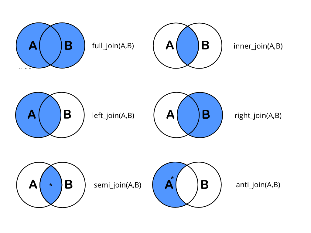
dplyr::_join

以資料在檔案第 5 章的 survVATrial.csv 為例, 隨機從前 10 位個體抽取 7 位, 進行 2 次, 得到 2 組資料 x 與 y. x 資料包函 id, treat, time,age.y資料包函id,cellcode,ceosor,age`.

## _join()
set.seed(1)
df <- dd %>% 
  select(treat, cellcode, time, censor, age) %>% 
  mutate(id = 1:n()) %>%
  filter(id <= 10) 
x <- df %>% 
  select(id, treat, time, age) %>% 
  sample_n(size = 7, replace = FALSE) %>%
  arrange(id)
y <- df %>% 
  select(id, cellcode, censor, age) %>% 
  sample_n(size = 7, replace = FALSE)  %>%
  arrange(id)
x
## # A tibble: 7 x 4
##      id treat    time   age
##   <int> <fct>   <int> <int>
## 1     1 placebo    72    69
## 2     2 placebo   411    64
## 3     3 placebo   228    38
## 4     4 placebo   126    63
## 5     5 placebo   118    65
## 6     7 placebo    82    69
## 7     9 placebo   314    43
y
## # A tibble: 7 x 4
##      id cellcode censor     age
##   <int> <fct>    <fct>    <int>
## 1     1 squamous dead        69
## 2     2 squamous dead        64
## 3     3 squamous dead        38
## 4     5 squamous dead        65
## 5     6 squamous dead        49
## 6     7 squamous dead        69
## 7    10 squamous survival    70
inner_join(x, y)
## # A tibble: 5 x 6
##      id treat    time   age cellcode censor
##   <int> <fct>   <int> <int> <fct>    <fct> 
## 1     1 placebo    72    69 squamous dead  
## 2     2 placebo   411    64 squamous dead  
## 3     3 placebo   228    38 squamous dead  
## 4     5 placebo   118    65 squamous dead  
## 5     7 placebo    82    69 squamous dead
left_join(x, y) 
## # A tibble: 7 x 6
##      id treat    time   age cellcode censor
##   <int> <fct>   <int> <int> <fct>    <fct> 
## 1     1 placebo    72    69 squamous dead  
## 2     2 placebo   411    64 squamous dead  
## 3     3 placebo   228    38 squamous dead  
## 4     4 placebo   126    63 <NA>     <NA>  
## 5     5 placebo   118    65 squamous dead  
## 6     7 placebo    82    69 squamous dead  
## 7     9 placebo   314    43 <NA>     <NA>
right_join(x, y)
## # A tibble: 7 x 6
##      id treat    time   age cellcode censor  
##   <int> <fct>   <int> <int> <fct>    <fct>   
## 1     1 placebo    72    69 squamous dead    
## 2     2 placebo   411    64 squamous dead    
## 3     3 placebo   228    38 squamous dead    
## 4     5 placebo   118    65 squamous dead    
## 5     7 placebo    82    69 squamous dead    
## 6     6 <NA>       NA    49 squamous dead    
## 7    10 <NA>       NA    70 squamous survival
full_join(x, y) 
## # A tibble: 9 x 6
##      id treat    time   age cellcode censor  
##   <int> <fct>   <int> <int> <fct>    <fct>   
## 1     1 placebo    72    69 squamous dead    
## 2     2 placebo   411    64 squamous dead    
## 3     3 placebo   228    38 squamous dead    
## 4     4 placebo   126    63 <NA>     <NA>    
## 5     5 placebo   118    65 squamous dead    
## 6     7 placebo    82    69 squamous dead    
## 7     9 placebo   314    43 <NA>     <NA>    
## 8     6 <NA>       NA    49 squamous dead    
## 9    10 <NA>       NA    70 squamous survival
semi_join(x, y) 
## # A tibble: 5 x 4
##      id treat    time   age
##   <int> <fct>   <int> <int>
## 1     1 placebo    72    69
## 2     2 placebo   411    64
## 3     3 placebo   228    38
## 4     5 placebo   118    65
## 5     7 placebo    82    69
anti_join(x, y) 
## # A tibble: 2 x 4
##      id treat    time   age
##   <int> <fct>   <int> <int>
## 1     4 placebo   126    63
## 2     9 placebo   314    43