Part 5 Support Vector Machines
I mentioned two chapters back that I constructed two variants of this classification algorithm: one with a radial kernel and one with a linear kernel.
If none of the above makes sense, I will explain what these are in this chapter of the document.
5.1 What is a Support Vector Machine?
Support Vector Machines (i.e., SVMs) are a kind of supervised machine learning algorithm that is used for classification (and also regression) problems (e.g., given a set of features, can you predict whether or not sample A is of which class of data).
The way a SVM does classification is via hyperplanes - a plane in one less the dimension of the data (e.g., if your data had three dimensions, a SVM would attempt to divide your data via 2D lines). But, to be more specific, a SVM works by finding a hyperplane in your data’s dimension that distinctly classifies all of the data points into two or more categories.
I think we should start off with a simple example of how an SVM could be done.
5.2 Linearly Separable Data
Suppose that I want to classify Iris species into two species: setosa and virginica based on the length and widths of their petals:
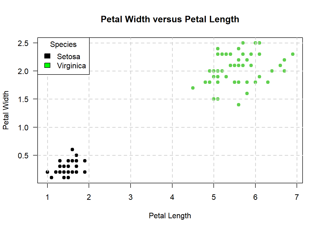
It is apparent from the above graph that one way I could go about doing this with a support vector machine is to draw diagonal lines like so:
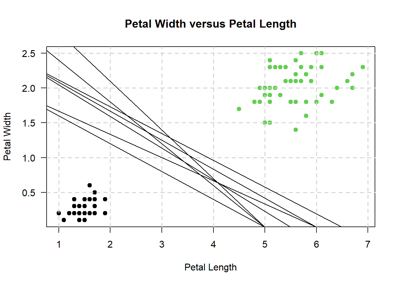
However, which line actually gets picked in the end? The line that maximizes the distances between the two nearest data points of each class will end up getting picked - so, our support vector machine might end up looking something like this:
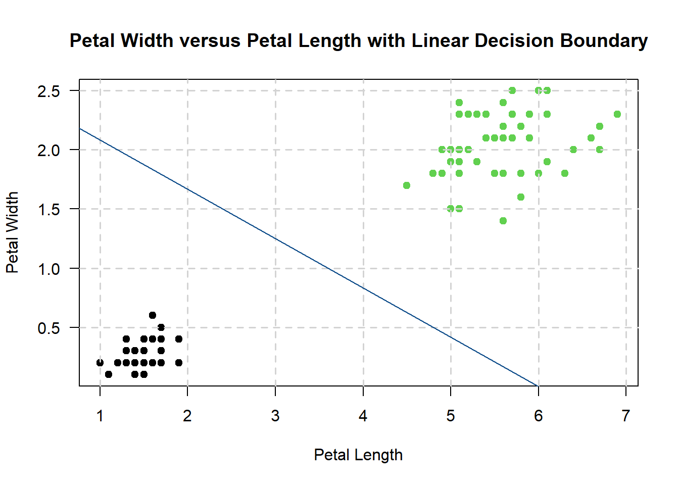
Granted - this may not be the most accurate depiction of a support vector machine, but the diagonal line is called the decision boundary. Anything that falls below the decision boundary is determined to be of class setosa; anything that falls above is of class virginica.
Furthermore, the points that lie the closest to the decision boundary are called the support vectors. The distance between the support vectors and the decision boundary is called the margin.
The main idea is that the further away the support vectors are from the decision boundary, the higher the probability that the SVM will correctly classify the points into their correct classes. The support vectors themselves are crucial for this step: since the SVM algorithm aims to maximize the distance between the decision boundary and the support vectors, a change in the support vectors’ position can shift the decision boundary!
5.2.1 What if we had data that looked like this (see below)?
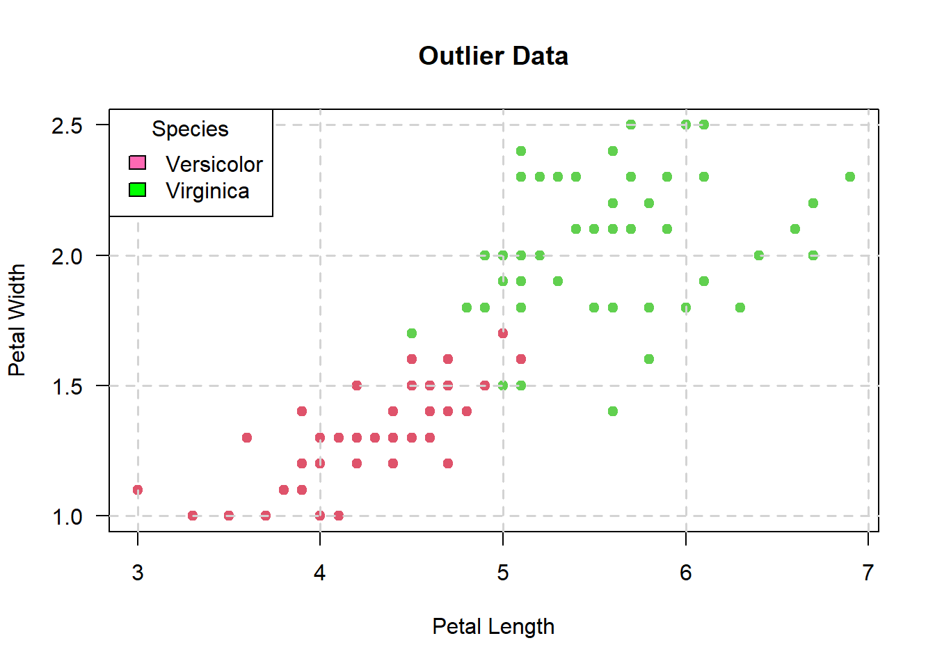
There are a couple of pink points in the above plot that look like they’re in the region of the scatterplot with green points.
Nevertheless, such points are considered “outliers” in the support vector machine algorithm - one of the perks of using a SVM is that the algorithm is resistant to outliers.
That said, is the roughly what the linear SVM would look like:
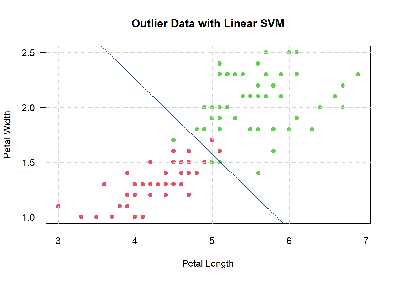
So, the linear SVM performs the same as before (i.e., data without outliers), albeit for each point in the pink area that crosses the decision boundary (i.e., the blue line), a penalty term is added to the hyperplane’s equation.
If you are interested in what these penalties are, I have included a fair chunk of the mathematics behind SVMs at the back of this chapter.
5.3 Non-Linearly Separable Data
Suppose that we have data that looks like this:
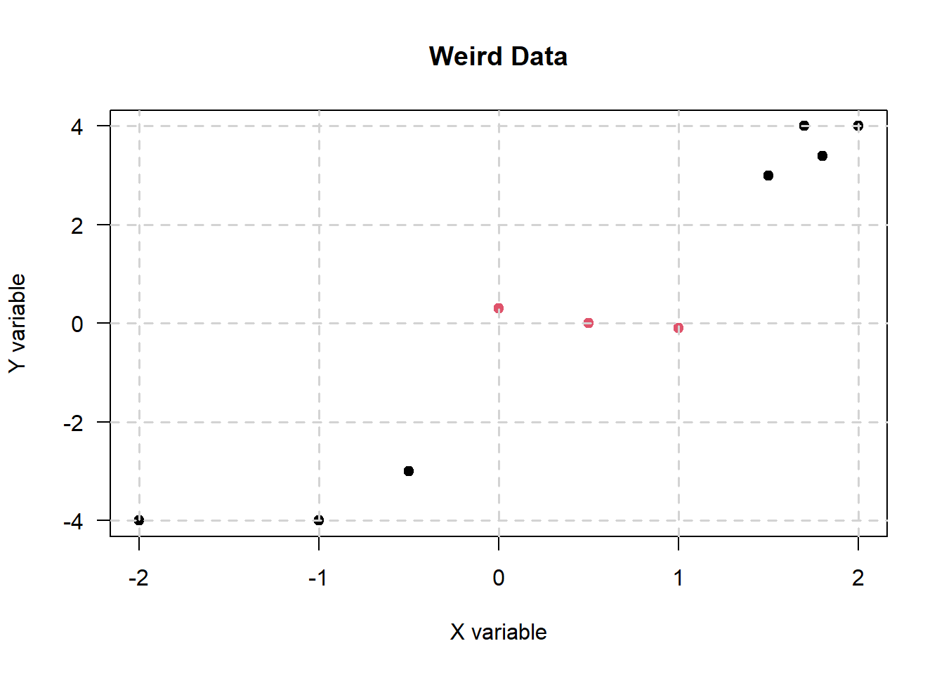
It is clear that we cannot use a linear decision boundary to divide the data. However, the points still look like they’re clustered well - hence, what the SVM algorithm might do is to add a third dimension.
Up until now, there were two dimensions: \(X\) and \(Y\). In the SVM algorithm, the kernel function transforms the data into a higher dimension - in this case, the third dimension - \(Z\).
For the sake of simplicity, let’s suppose that the kernel maps the data via the equation of a paraboloid:
\[\begin{equation} z = \frac{x^2}{a^2} + \frac{y^2}{b^2} \tag{5.1} \end{equation}\]
Note that equation (5.1) is also the equation of a circle for \(a = 1\) and \(b = 1\)!
Nonetheless, when projected onto three dimensions, the data looks something like this:
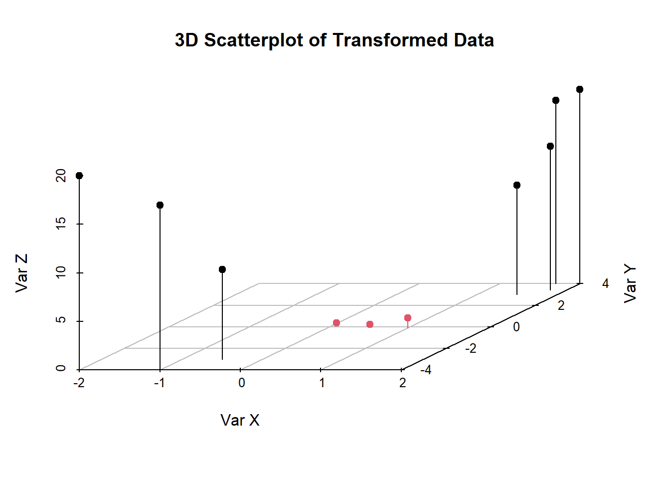
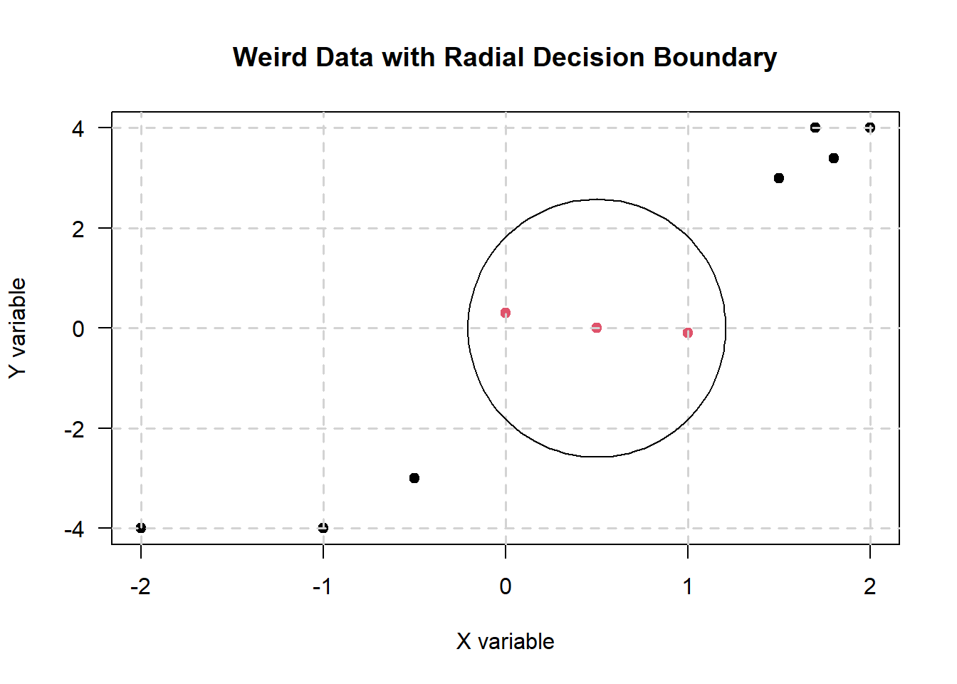
From here, it looks like we can draw a hyperplane at \(Z = 5\) or something along the lines. Hence, substituting \(Z = 5\) for equation (5.1), we get the circular decision boundary:
\[\begin{equation} x^2 + y^2 = 5 \end{equation}\]
Hence, the decision boundary looks something like this on the 2D scatterplot (not accurate - just a rough drawing I quickly whipped up in base R):
5.4 Kernel Trick
While we can use equations like (5.1) to map our data to higher dimensions, doing so is computationally expensive and also time-consuming, especially if you have a large amount of data to deal with.
Hence, enter the kernel trick: a way of computing the dot product (in case you’ve forgotten your high-school Linear Algebra) between two vectors \(x\) and \(y\) as a faster alternative to mapping the data like I did in equation (5.1).
There are also different kernels that can be used - this is also what the kernel parameter in tune.svm() does: it determines which kernel e1071 will apply to the data. I will talk about the mathematics behind the radial and the linear kernel trick in the Kernels section.
Nevertheless, let’s go back to the example used in the previous sub-section (i.e., the “Weird Data”). The transformation to the third dimension \(Z\) is denoted by equation (5.1).
Hence, suppose that we have two vectors \(a\) and \(b\) such that:
\[\begin{align} a = \left[ \begin{array}{c} x_a \\ y_a \\ z_a \end{array} \right] && b = \left[ \begin{array}{c} x_b \\ y_b \\ z_b \end{array} \right] \end{align}\]
Hence, the dot product \(a \cdot b\) is:
\[\begin{align} a \cdot b &= x_ax_b + y_ay_b + z_az_b \\ &= x_ax_b + y_ay_b + ({x_a}^2 + {y_a}^2) \times ({x_b}^2 + {y_b}^2) \end{align}\]
Thereafter, the support vector machine will then determine the best hyperplane to construct a decision boundary with, albeit with the dot product.
5.5 Advanced Stuff
Everything here is more theoretical and mathematical. Kudos to you if can read it all and understand it, but if not, don’t sweat it.
5.5.1 Equation of a hyperplane
Earlier in this chapter, I mentioned that support vector machines use hyperplanes to classify data into one or more categories of samples.
Well, suppose that we have a dataset of \(m\) dimensions, a set of vectors \(W_i\) for \(i \in [0, m]\), and a biased term \(b = W_0\). Hence, the equation of a hyperplane \(y\) in \(m\) dimensions is:
\[\begin{align} y &= W_0 + W_1X_1 + W_2X_2 + W_3X_3 + ... \\ &= W_0 + \sum_{i = 1}{m}W_ix_i \\ &= W_0 + W^TX \\ &= b + w^TX \tag{5.2} \end{align}\]
Where:
- \(W_i\) are vectors.
- \(b\) is the biased term.
- \(X\) are the variables.
5.5.2 Hard and soft margins
Near the beginning of this chapter, I mentioned something about a “penalty term” being added to the hyperplane’s equation for each point that is not classified correctly (i.e., outlier data).
However, to understand what this means, we need to talk a little about hard and soft margins.
5.5.2.1 Hard margins
Consider this plot once again, albeit with three hyperplanes \(\alpha\), \(\beta\), and \(\gamma\):
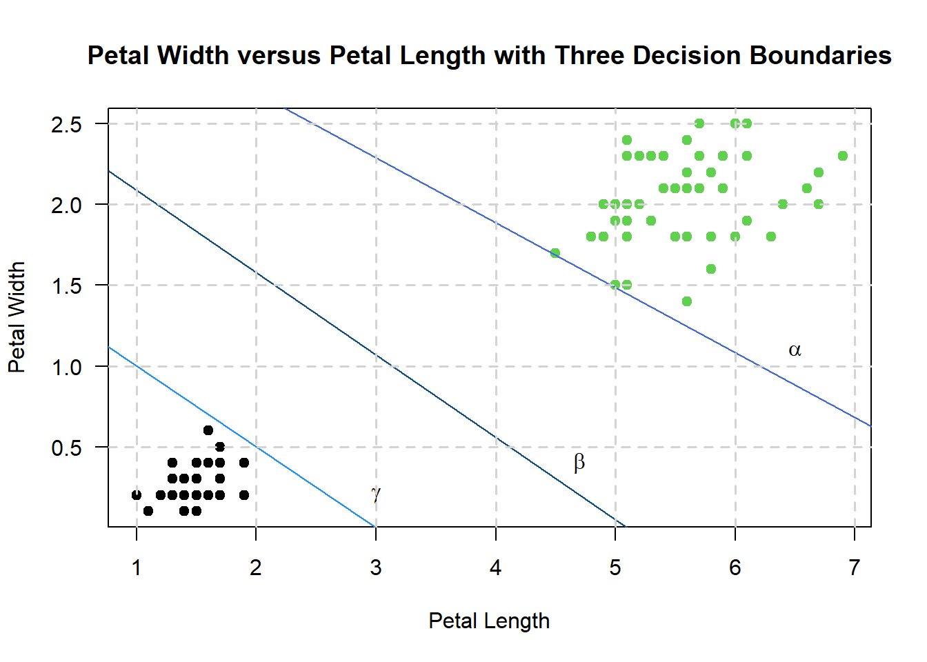
And we can define the following hyperplanes \(\alpha\), \(\beta\), and \(\gamma\) as:
\[\begin{align} \beta &: b + W^TX = 0 \\ \alpha &: b + W^TX = 1 \\ \gamma &: b + W^TX = -1 \end{align}\]
Thereafter, define \(\beta\) as the original decision boundary, everything above \(\alpha\) as the positive domain of the scatterplot, and everything below \(\gamma\) as the negative domain of the scatterplot.
Hence, for a point \(X_i\) that lies on the decision boundary, we say that:
\[\begin{align} y_i &= 1 \\ y_i(W^TX_i + b) &= 1 \end{align}\]
When a point lies away from the hyperplane in the positive domain, then:
\[\begin{align} y_i &= 1 \\ y_i(W^TX_i + b) &> 1 \end{align}\]
And when it lies on the hyperplane \(\gamma\), then:
\[\begin{align} y_i &= -1 \\ y_i(W^TX_i + b) &= 1 \end{align}\]
Otherwise, if the point lies in the negative domain away from the hyperplane, then:
\[\begin{align} y_i &= -1 \\ y_i(W^TX_i + b) &> 1 \end{align}\]
Hence, from the above equations, a point \(i\) is mis-classified if \(y_i(W^TXi + b) < 1\)
SVMs that obey the above property are called hard margin SVMs. This is because any outlier in the data would render the SVM unable to classify each and every point (also an assumption of hard margin SVMs).
5.5.2.2 Soft margins
In the first example, I assume that the data is linearly separable (i.e., they can be separated via a linear hyperplane), but this isn’t always the case for all data (especially the second example), especailly real-world data!
Hence, we can update the equality \(y_i(W^TXi + b) < 1\) to include a slack variable \(\xi_i\) to yield:
\[\begin{equation} y_i(W^TX_i + b) \ge 1 - \xi_i \end{equation}\]
When \(\xi_i = 0\), then all points can be considered as correctly classified. Otherwise, if \(\xi_i > 0\), then we have incorrectly classified points.
One way to think about \(\xi_i\) is as an “error” term that is associated with each variable. The average error then is:
\[\begin{equation} \frac{1}{n} = \sum_{i = 1}{n}\xi_i \end{equation}\]
And our objective function is:
\[\begin{equation} \min{\left(\frac{1}{2}||w||^2 + \sum_{i = 1}^{n}\xi_i \right)} \end{equation}\]
Subject to the following constraint:
\[\begin{equation} y_i(W^TX + b) \ge 1 - \xi_i \text{ for all } i \in [1, n] \end{equation}\]
5.5.3 Kernels
Think of a kernel as a way to represent your data so that it allows you to compare data points in some higher dimensional space.
5.5.3.1 Properties of a kernel
I’ve pulled the contents of this section off a link from Princeton University - nevertheless, suppose that we have the following:
Definition 5.1 (Kernel Function) Given some abstract space \(X\) (e.g., documents, images, proteins, etc.), the function \(\kappa\): \(X \times X \to \mathbb{R}\) is called a kernel function.
Kernel functions are also used to quantify differences between two pairs of objects in \(X\) - a kernel function also has two properties:
It is symmetric
\(\forall x, x' \in X, \kappa(x, x') = \kappa(x', x)\)
It is non-negative
\(\forall x, x' \in X, \kappa(x, x') \ge 0\)
Or in layman terms, for any two pair of points \(x\) and \(x'\) in the data \(X\), the results of the calling the kernel functions \(\kappa(x, x')\) and \(\kappa(x', x)\) are the same. Furthermore, the mapped data point (to a higher dimension) using \(\kappa\) results in a value greater than or equal to zero.
5.5.3.2 Linear kernels
Here, the kernel function \(\kappa(x, x')\) is denoted as the dot product between two vectors - in other words:
\[\begin{equation} \kappa(x, x') = x^Tx' \end{equation}\]
Linear kernels map the data to the same dimensional space as the data. In our case, it looks like there’s a clear separation between treated and control subjects - hence, I didn’t think it was necessary to map our data to a higher dimensional space.
5.5.3.3 Gaussian kernels
The Gaussian kernel (or the radial basis function - what e1071 refers to as radial) is denoted by:
\[\begin{equation} \kappa(x, x') = \exp{\left(-\frac{1}{2}(x - x')^T \times \Sigma^{-1}(x - x')\right)} \end{equation}\]
Where \(\Sigma\) is the covariance matrix of all variables in the data.