Part 3 My Code

I will admit: I have used packages and techniques that go beyond the scope of BS0004.

For this reason, there are many sections to this .html document that you’re currently reading. In those sections, I attempt to elaborate on parts of the workflow that are not covered by professors Wilson or Jarkko.

3.1 Setting Up the Working Environment

I first set the working directory of my current R session to my laptop’s “Downloads” folder:

setwd("C:/Users/Kevin/Downloads")

I then loaded in the following packages:

library(tidyverse) ; library(pheatmap) ; library(ggplot2)
library(ROCR) ; library(caret) ; library(e1071)
library(gprofiler2) ; library(corrplot) ; library(vip)

I will not elaborate on what the ggplot2 or what the pheatmap package does. These have already been explained in lectures 5 and onwards.

Nonetheless:

The tidyverse packages are a collection packages authored by Hadley Wickham that obey his tidy data principle. While not technically a part of the tidyverse, calling library(tidyverse) loads in the magrittr package. The biggest boon of magrittr is the pipe %>%. The tidyverse packages are (in no particular order):
- stringr: this package is for string processing.
- tidyr: this is used for tidying up data.
- dplyr: this is used for data manipulation.
- readr: this is used for reading in data.
- purrr: this is used for functional programming.
I used the ROCR package to plot the ROC curves of the various supervised clustering models and calculate their AUCs.
I used the caret package to not only train the majority of the supervised clustering models, but also perform k-fold cross validation.
I used the e1071 package to create a linear support vector machine.
I used the gprofiler2 package to perform GO term analysis. This package has been endorsed by the Gene Ontology.
I used the corrplot package to generate aesthetically-pleasing correlation matrices.
I used the vip package to generate variable importance plots.

3.2 Exploring the Data

While I am not sure what has been done to the data to clean it (do ask Sean - he was the one who sent me the data in a .csv file), I began by reading the data into my current R session:

data <- read.csv("original idea.csv")

I then decided to transpose the original data frame and save the transposed data frame in a variable called transposed. While I was at this, I also changed the row and column names of transposed to the column and row names of data respectively:

row <- data[, 1] ; data <- data[, -1] ; col <- colnames(data)
transposed <- data %>% t() %>% as.data.frame() 
colnames(transposed) <- row ; rownames(transposed) <- col

I also created a new variable in transposed called Status: a factor that states whether or not a sample (i.e., patient) is a control or has been treated:

transposed$Status <- c(rep("Control", 2), rep("Treated", 4), rep("Control", 10), rep("Treated", 8))
transposed$Status <- as.factor(transposed$Status)

In the next several sections, I then performed some exploratory data analysis prior to actually building the supervised classifiers. I’ve also constructed numerous plots during this step of the workflow.

3.2.1 A heatmap using `pheatmap()`

I made a heatmap using all the genes as suggested by Sean:

pheatmap(transposed[, 1:(ncol(transposed) - 1)], scale = "column", show_colnames = FALSE)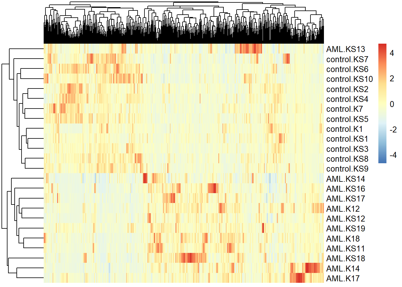

The heatmap seems to suggest that there are definite differences between treated individuals and controls.

3.2.1.1 Performing a little GO-term analysis

GO term analysis is generally conducted after differential expression analysis, but since the link to the data Sean provided did not have a count matrix (nor do I have the means to generate one as I do not have the .fastq or the SAM / BAM files for the data), there was just no way for me to conform to the traditional workflow.

Nevertheless, I thought that it would still be interesting to have a feel for what cellular processes are the most affected as a result of the above heatmap. Hence, I conducted a GO term analysis to see if anything would pop up.

Note that in the below code block, I set organism to hsapiens as we’re dealing with human samples here. All annotations for the genes come from EnsemblGenomes (i.e., “ENSG” - this is the default database that gconvert() will search) - the results of below code block has been saved into a variable called GOresults:

GOresults <- gconvert(colnames(transposed), organism = "hsapiens", target = "ENSG")

The contents of GOresults (not including the first three columns) are shown below:

Table 3.1: Results of GO Term Analysis on bestGenes
target	name	description	namespace
ENSG00000198997	MIR107	microRNA 107 [Source:HGNC Symbol;Acc:HGNC:31496]	MIRBASE
ENSG00000221783	MIR1183	microRNA 1183 [Source:HGNC Symbol;Acc:HGNC:35264]	MIRBASE
ENSG00000221745	MIR1197	microRNA 1197 [Source:HGNC Symbol;Acc:HGNC:35376]	MIRBASE
ENSG00000283203	MIR1246	microRNA 1246 [Source:HGNC Symbol;Acc:HGNC:35312]	MIRBASE
ENSG00000283958	MIR1248	microRNA 1248 [Source:HGNC Symbol;Acc:HGNC:35314]	MIRBASE
ENSG00000221598	MIR1249	microRNA 1249 [Source:HGNC Symbol;Acc:HGNC:35315]	MIRBASE
ENSG00000221265	MIR1255A	microRNA 1255a [Source:HGNC Symbol;Acc:HGNC:35320]	MIRBASE
ENSG00000221754	MIR1260A	microRNA 1260a [Source:HGNC Symbol;Acc:HGNC:35325]	MIRBASE
ENSG00000266192	MIR1260B	microRNA 1260b [Source:HGNC Symbol;Acc:HGNC:38258]	MIRBASE
ENSG00000221680	MIR1278	microRNA 1278 [Source:HGNC Symbol;Acc:HGNC:35356]	MIRBASE
ENSG00000221264	MIR1284	microRNA 1284 [Source:HGNC Symbol;Acc:HGNC:35362]	MIRBASE
ENSG00000281842	MIR1291	microRNA 1291 [Source:HGNC Symbol;Acc:HGNC:35284]	MIRBASE
ENSG00000221430	MIR1294	microRNA 1294 [Source:HGNC Symbol;Acc:HGNC:35287]	MIRBASE
ENSG00000275377	MIR1299	microRNA 1299 [Source:HGNC Symbol;Acc:HGNC:35290]	MIRBASE
ENSG00000221552	MIR1303	microRNA 1303 [Source:HGNC Symbol;Acc:HGNC:35301]	MIRBASE
ENSG00000223109	MIR1538	microRNA 1538 [Source:HGNC Symbol;Acc:HGNC:35382]	MIRBASE
ENSG00000207695	MIR184	microRNA 184 [Source:HGNC Symbol;Acc:HGNC:31555]	MIRBASE
ENSG00000215938	MIR190B	microRNA 190b [Source:HGNC Symbol;Acc:HGNC:33656]	MIRBASE
ENSG00000238705	MIR1976	microRNA 1976 [Source:HGNC Symbol;Acc:HGNC:37064]	MIRBASE
ENSG00000207568	MIR203A	microRNA 203a [Source:HGNC Symbol;Acc:HGNC:31581]	MIRBASE
ENSG00000207604	MIR206	microRNA 206 [Source:HGNC Symbol;Acc:HGNC:31584]	MIRBASE
ENSG00000284442	MIR2110	microRNA 2110 [Source:HGNC Symbol;Acc:HGNC:37071]	MIRBASE
ENSG00000212102	MIR301B	microRNA 301b [Source:HGNC Symbol;Acc:HGNC:33667]	MIRBASE
ENSG00000265396	MIR3128	microRNA 3128 [Source:HGNC Symbol;Acc:HGNC:38188]	MIRBASE
ENSG00000264931	MIR3138	microRNA 3138 [Source:HGNC Symbol;Acc:HGNC:38341]	MIRBASE
ENSG00000264823	MIR3154	microRNA 3154 [Source:HGNC Symbol;Acc:HGNC:38176]	MIRBASE
ENSG00000264226	MIR3168	microRNA 3168 [Source:HGNC Symbol;Acc:HGNC:38249]	MIRBASE
ENSG00000199090	MIR326	microRNA 326 [Source:HGNC Symbol;Acc:HGNC:31769]	MIRBASE
ENSG00000284186	MIR3615	microRNA 3615 [Source:HGNC Symbol;Acc:HGNC:38905]	MIRBASE
ENSG00000198973	MIR375	microRNA 375 [Source:HGNC Symbol;Acc:HGNC:31868]	MIRBASE
ENSG00000264803	MIR378C	microRNA 378c [Source:HGNC Symbol;Acc:HGNC:38374]	MIRBASE
ENSG00000263831	MIR378E	microRNA 378e [Source:HGNC Symbol;Acc:HGNC:41671]	MIRBASE
ENSG00000283829	MIR378I	microRNA 378i [Source:HGNC Symbol;Acc:HGNC:41620]	MIRBASE
ENSG00000266320	MIR3909	microRNA 3909 [Source:HGNC Symbol;Acc:HGNC:38987]	MIRBASE
ENSG00000263885	MIR3920	microRNA 3920 [Source:HGNC Symbol;Acc:HGNC:38974]	MIRBASE
ENSG00000202566	MIR421	microRNA 421 [Source:HGNC Symbol;Acc:HGNC:32793]	MIRBASE
ENSG00000199156	MIR422A	microRNA 422a [Source:HGNC Symbol;Acc:HGNC:31879]	MIRBASE
ENSG00000265483	MIR4443	microRNA 4443 [Source:HGNC Symbol;Acc:HGNC:41830]	MIRBASE
ENSG00000264408	MIR4470	microRNA 4470 [Source:HGNC Symbol;Acc:HGNC:41833]	MIRBASE
ENSG00000263790	MIR4473	microRNA 4473 [Source:HGNC Symbol;Acc:HGNC:41540]	MIRBASE
ENSG00000264712	MIR4504	microRNA 4504 [Source:HGNC Symbol;Acc:HGNC:41624]	MIRBASE
ENSG00000264737	MIR4511	microRNA 4511 [Source:HGNC Symbol;Acc:HGNC:41589]	MIRBASE
ENSG00000284565	MIR451A	microRNA 451a [Source:HGNC Symbol;Acc:HGNC:32053]	MIRBASE
ENSG00000266140	MIR4533	microRNA 4533 [Source:HGNC Symbol;Acc:HGNC:41886]	MIRBASE
ENSG00000271898	MIR4791	microRNA 4791 [Source:HGNC Symbol;Acc:HGNC:41704]	MIRBASE
ENSG00000283736	MIR484	microRNA 484 [Source:HGNC Symbol;Acc:HGNC:32341]	MIRBASE
ENSG00000283726	MIR5193	microRNA 5193 [Source:HGNC Symbol;Acc:HGNC:43534]	MIRBASE
ENSG00000212040	MIR543	microRNA 543 [Source:HGNC Symbol;Acc:HGNC:33664]	MIRBASE
ENSG00000221333	MIR548K	microRNA 548k [Source:HGNC Symbol;Acc:HGNC:35285]	MIRBASE
ENSG00000212017	MIR548U	microRNA 548u [Source:HGNC Symbol;Acc:HGNC:38316]	MIRBASE
ENSG00000266721	MIR5695	microRNA 5695 [Source:HGNC Symbol;Acc:HGNC:43548]	MIRBASE
ENSG00000207627	MIR581	microRNA 581 [Source:HGNC Symbol;Acc:HGNC:32837]	MIRBASE
ENSG00000208022	MIR618	microRNA 618 [Source:HGNC Symbol;Acc:HGNC:32874]	MIRBASE
ENSG00000207631	MIR641	microRNA 641 [Source:HGNC Symbol;Acc:HGNC:32897]	MIRBASE
ENSG00000211575	MIR760	microRNA 760 [Source:HGNC Symbol;Acc:HGNC:33666]	MIRBASE
ENSG00000283880	MIR7704	microRNA 7704 [Source:HGNC Symbol;Acc:HGNC:50089]	MIRBASE
ENSG00000284160	MIR7706	microRNA 7706 [Source:HGNC Symbol;Acc:HGNC:50110]	MIRBASE
ENSG00000276083	MIR7976	microRNA 7976 [Source:HGNC Symbol;Acc:HGNC:50092]	MIRBASE

3.2.2 Constructing a correlation plot using `corrplot()`

I made a correlation matrix using the base R function cor() and the corrplot() function from the corrplot package.

I did this because I wanted to know if the data was reproducible - that is, whether or not they varied according to sample and treatment conditions.

In the previous correlation matrix I made, I accidentally used the wrong values - I should have used the samples’ (i.e., patients’) gene expression values instead:

data %>% cor() %>% corrplot(method = "square")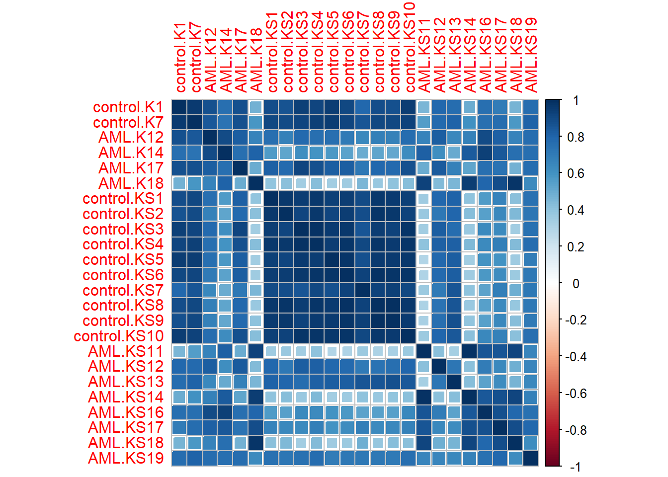

Almost immediately, it was clear that good number of samples are reproducible (i.e., patients whose gene expression values are more or less the same) across different treatment conditions.

3.3 Perfoming PCA

Given the amount of genes in transposed and the above correlation matrix, it was apparent that PCA had to be done.

Training the models using all of the genes in transposed would have taken far too long, not to mention that it is impossible to visualize the gene expression values in 500+ dimensions.

Hence, I performed PCA via the base R function prcomp():

PCAdata <- transposed %>% select(-Status) %>% prcomp(scale. = TRUE)

And from this, I made two plots - a PCA plot using ggplot2:

ggplot(as.data.frame(PCAdata$x), aes(x = PCAdata$x[, 1], y = PCAdata$x[, 2])) + 
  geom_point(aes(col = transposed$Status)) +
  labs(title = "PCA Plot of Cancer Data",
       x = "PC1",
       y = "PC2") + scale_color_discrete(name = "Status")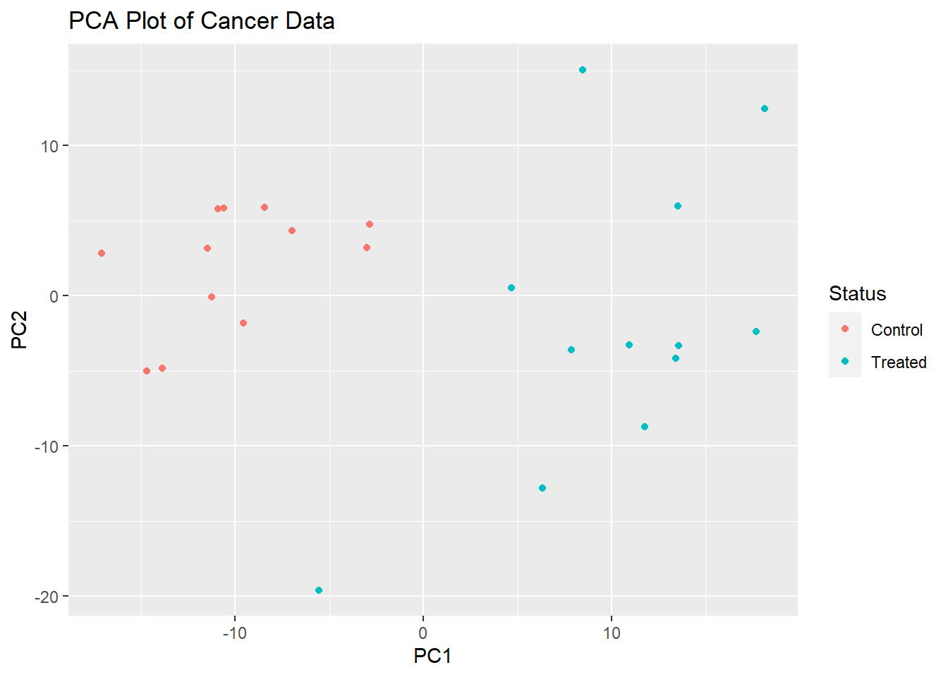

And a screeplot using the base R function barplot():

(PCAdata$x^2 / sum(PCAdata$x^2)) %>% as.data.frame() %>% colSums() %>% 
  barplot(main = "Screeplot of Transformed Data", 
          xlab = "Principal Component", 
          ylab = "Proportion of Explained Variance", las = 1, 
          col = "slategray2", ylim = c(0, 0.30))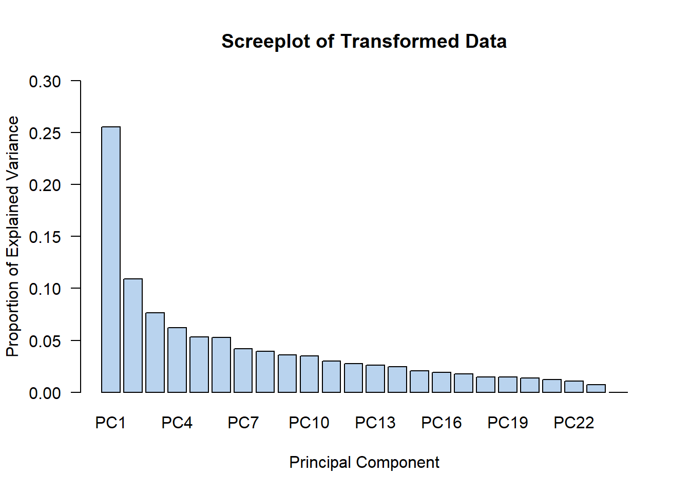

I personally thought that since PC1 and PC2 contained the highest explained variances out of all principal components (this is to be expected anyways), that we could go ahead and PC1 and PC2 to train our machine learning classifiers on.

3.4 Training the Models

3.4.1 Making the training and testing data

For this bit, I took the principal components from PCAdata. I then decided to combine them into a dataframe toUse via the cbind() function.

I also renamed a column using the rename() function from dplyr:

toUse <- cbind(PCAdata$x, transposed$Status) %>% as.data.frame() 
toUse$Status <- toUse[, ncol(toUse)] ; toUse[, ncol(toUse)] <- NULL 
toUse[, ncol(toUse)] <- as.factor(toUse[, ncol(toUse)])
toUse <- toUse %>% rename(Status = `V25`)

I also included the statuses of the patients in toUse.

I then made my training and testing sets via the createDataPartition() function - I also checked the dimensions of my training and testing sets of data using the dim() function:

set.seed(123)
index <- createDataPartition(toUse$Status, p = 0.6, list = FALSE)
training <- toUse[index, ] ; testing <- toUse[-index, ]
dim(training) ; dim(testing)

## [1] 16 25

## [1]  8 25

Note that the set.seed() function was used to ensure reproducibility! The value inside set.seed() can be anything as long as it is numeric.

3.4.2 Performing cross validation

Thereafter, I used the trainControl() function to perform a 10-fold cross validation (as this is the most common value of “k” in k-fold cross validation) - I saved the results of trainControl() in a variable called kfold:

kfold <- trainControl(method = "cv", n = 10)

3.4.3 Training the models

I trained several classification models according - the source code for their training are shown for a:

1) kNN algorithm

kNN <- train(Status ~ PC1 + PC2, data = training, method = "knn", trControl = kfold) %>% suppressWarnings()

2) linear support vector machine

linearSVM <- tune.svm(Status ~ ., data = training, kernel = "linear")

I also managed to construct a visual representation of the support vector machine:

plot(linearSVM$best.model, data = training, PC2 ~ PC1)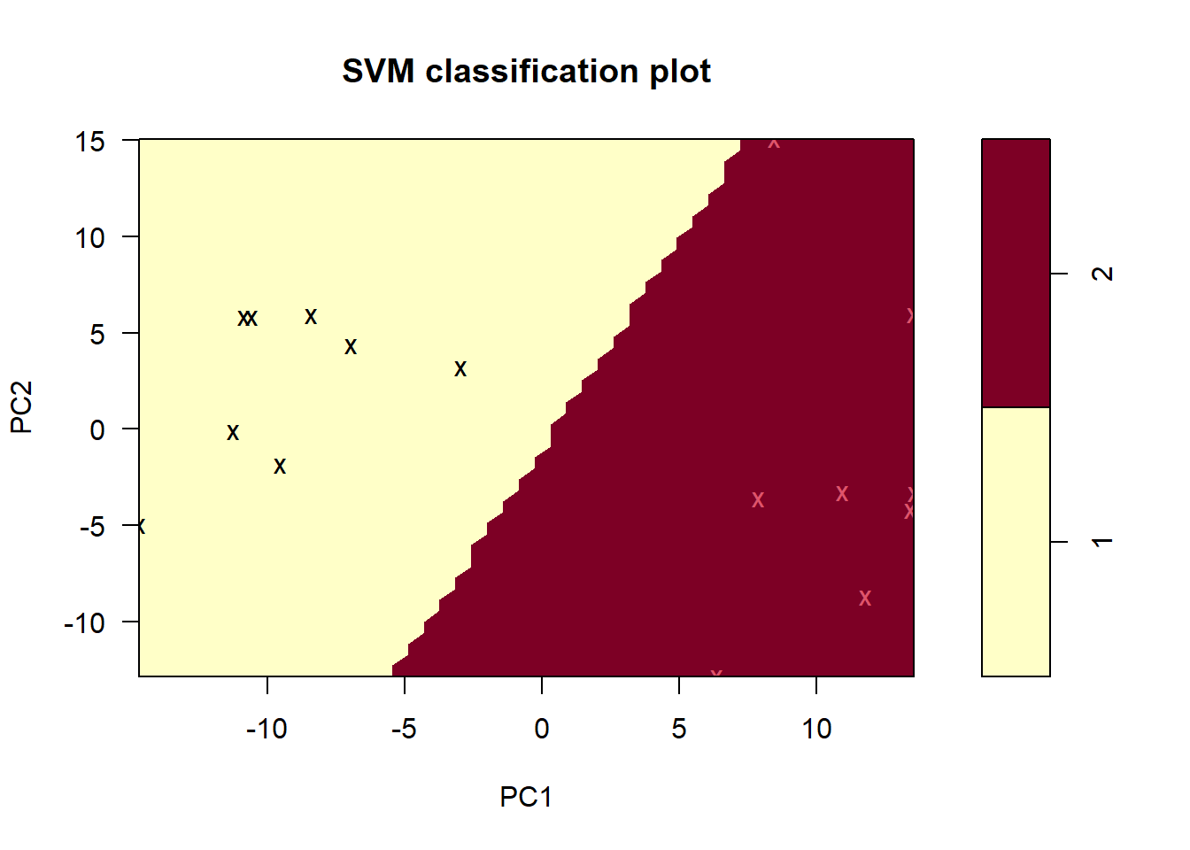

3) Radial support vector machine**

radialSVM <- tune.svm(Status ~ ., data = training, kernel = "radial")

And its plot:

plot(radialSVM$best.model, data = training, PC2 ~ PC1)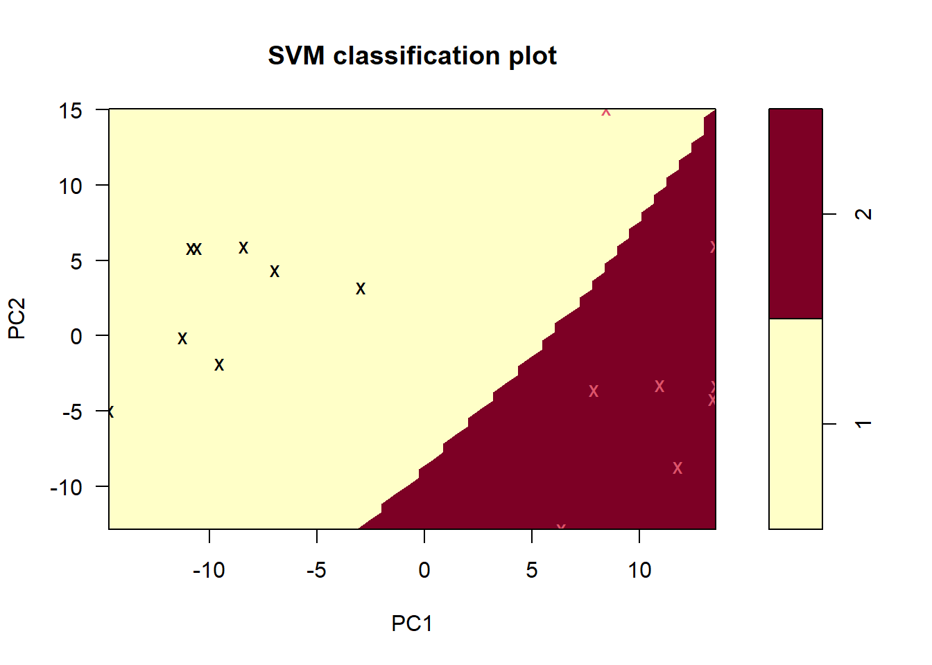

4) Decision tree

rpart <- train(Status ~ ., data = training, method = "rpart", 
               control = rpart::rpart.control(minsplit = 1),
               trControl = kfold) %>% suppressWarnings()

I purposely set minsplit to 1 in the control parameter. This is because we have a very small sample size - the minsplit parameter determines how many samples a split in the tree must benefit before the split is introduced as part of the model.

Nevertheless, the decision tree is shown below (NB: “2” are the treated samples):

rattle::fancyRpartPlot(rpart$finalModel)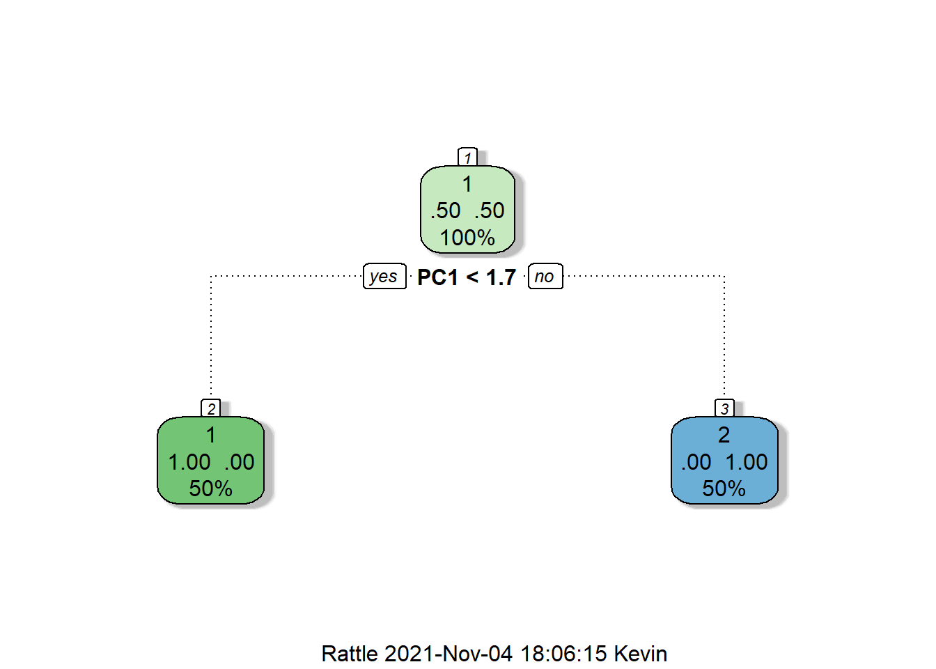

Out of curiousity, I also decided to make a variable importance plot to which principal components actually play a huge role in splitting the tree:

features <- vip(rpart, geom = "point", num_features = 24)
vip(rpart, geom = "point", num_features = 24)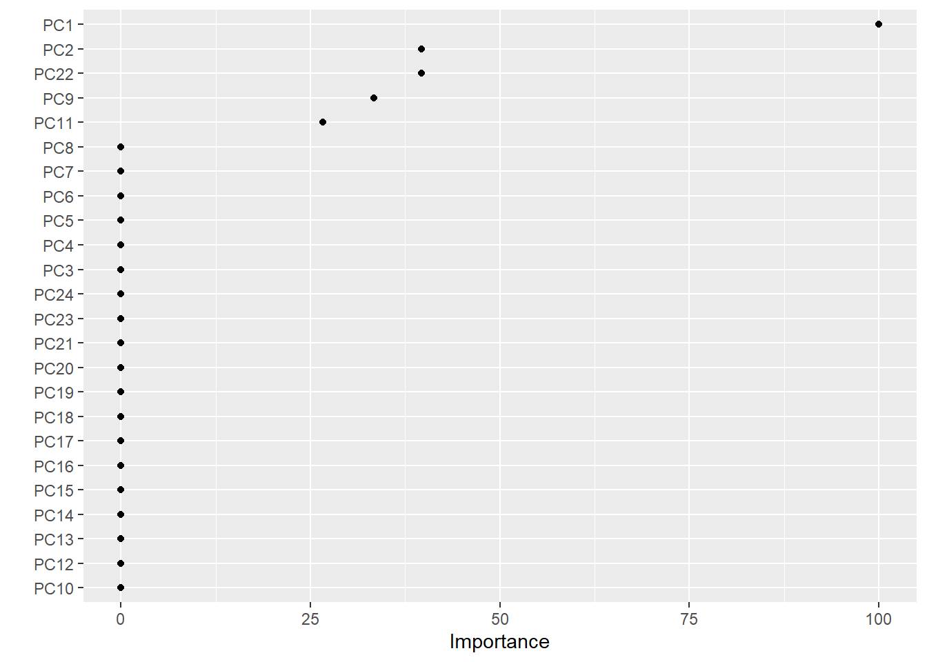

Principal components 1 and 2 were the features that had the highest variable importance. Out of curiosity, I then decided to retrain the model with the principal components that had a variable importance greater than 0:

feat <- features$data %>% filter(Importance > 0) %>% select(Variable) %>% unclass()
feat2 <- feat$Variable %>% paste(collapse = " + ")
rpart <- train(as.formula(paste0("Status ~ ", feat2)), data = training, method = "rpart", 
               control = rpart::rpart.control(minsplit = 1),
               trControl = kfold) %>% suppressWarnings()

And the decision tree looks like this:

rattle::fancyRpartPlot(rpart$finalModel)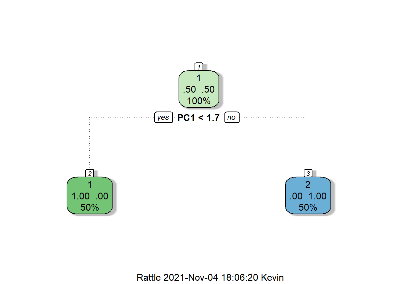

5) Ranger random forest

This is a supposedly “fast” variant of the original random forest algorithm:

ranger <- train(Status ~ ., data = training, method = "ranger", trControl = kfold) %>% suppressWarnings()

3.5 Evaluating the Models

I used the confusionMatrix() function from caret to generate a confusion matrix and from it, calculate the sensitivity (i.e., precision) and the recall of the model.

I also used the ROCR package to create a function plotROC() to not only plot the ROC curve of a model, but also calculate the AUC from the ROC curve:

plotROC <- function(model, testing, title) {
  AUCval <- predict(model, testing) %>% as.numeric() %>% 
    prediction(as.numeric(testing$Status)) %>% 
    performance(measure = "auc")
  AUCval <- AUCval@y.values[[1]]
  
  # Make the plot 
  predict(model, testing) %>% as.numeric() %>% 
    prediction(as.numeric(testing$Status)) %>% 
    performance("tpr", "fpr") %>% plot(main = paste0("ROC Curve of ", title),
                                       las = 1,
                                       colorize = TRUE)
  grid(lty = "dashed", lwd = 1.5) ; text(paste0("AUC = ", AUCval),
                                         x = 0.7, y = 0.3)
}

The performance() function is used to evaluate the model’s predictions against the actual results. The prediction() function is used to create an object of class prediction - while I am unsure why, this step is neccesary to generate ROC plots with ROCR!

Nevertheless, the models and their evaluations are:

1) kNN

kNNstats <- confusionMatrix(predict(kNN, testing), testing$Status)
kNNstats$byClass

##          Sensitivity          Specificity       Pos Pred Value 
##            1.0000000            0.7500000            0.8000000 
##       Neg Pred Value            Precision               Recall 
##            1.0000000            0.8000000            1.0000000 
##                   F1           Prevalence       Detection Rate 
##            0.8888889            0.5000000            0.5000000 
## Detection Prevalence    Balanced Accuracy 
##            0.6250000            0.8750000

The kNN’s confusion matrix is as such:

kNNstats$table

##           Reference
## Prediction 1 2
##          1 4 1
##          2 0 3

Also note the ROC curve and AUC:

plotROC(kNN, testing, "kNN")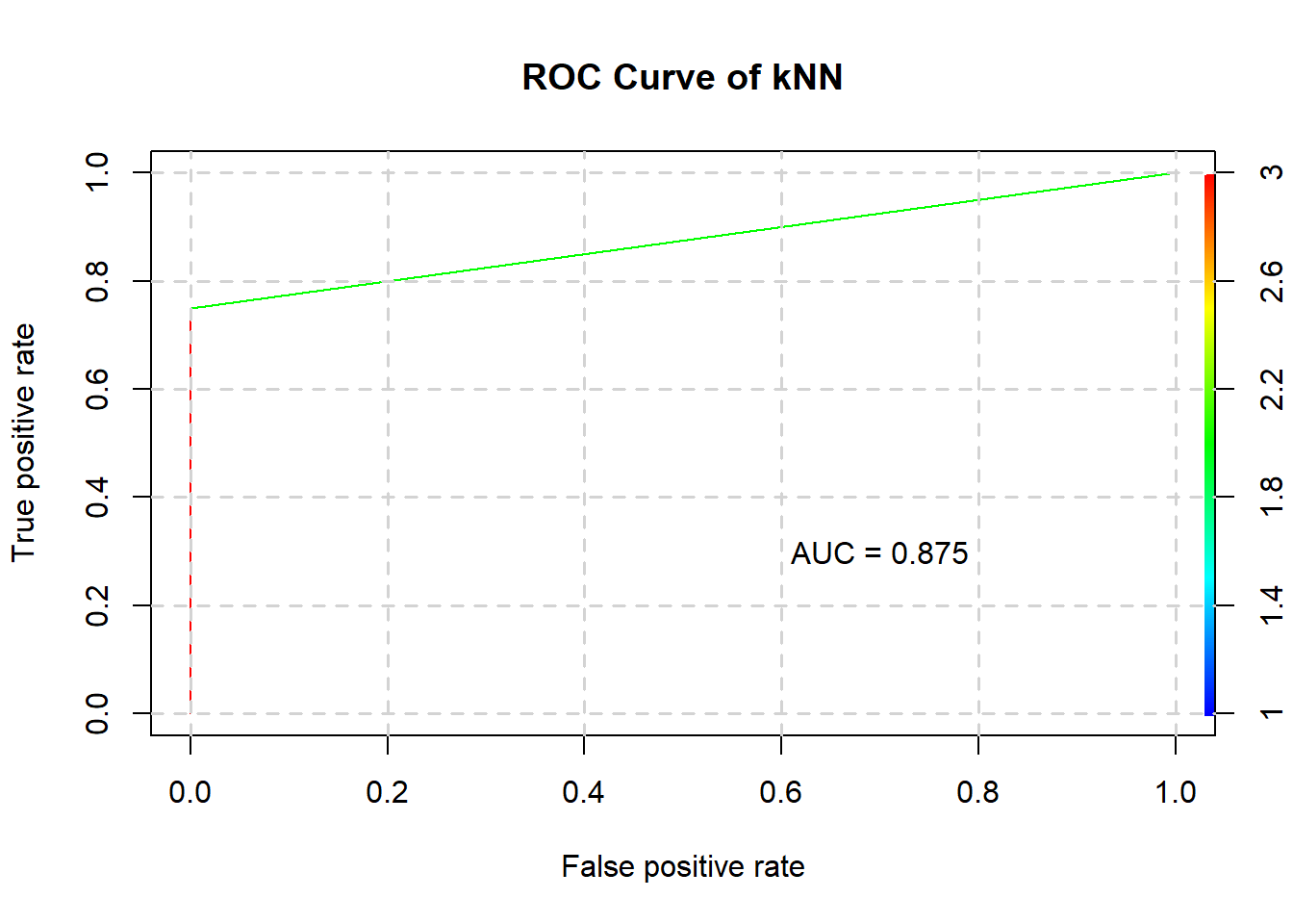

2) Linear support vector machine

linStats <- confusionMatrix(predict(linearSVM$best.model, testing), testing$Status)
linStats$byClass

##          Sensitivity          Specificity       Pos Pred Value 
##            1.0000000            0.5000000            0.6666667 
##       Neg Pred Value            Precision               Recall 
##            1.0000000            0.6666667            1.0000000 
##                   F1           Prevalence       Detection Rate 
##            0.8000000            0.5000000            0.5000000 
## Detection Prevalence    Balanced Accuracy 
##            0.7500000            0.7500000

The linear SVM’s confusion matrix is as such:

linStats$table

##           Reference
## Prediction 1 2
##          1 4 2
##          2 0 2

And its ROC curve and AUC:

plotROC(linearSVM$best.model, testing, "Linear SVM")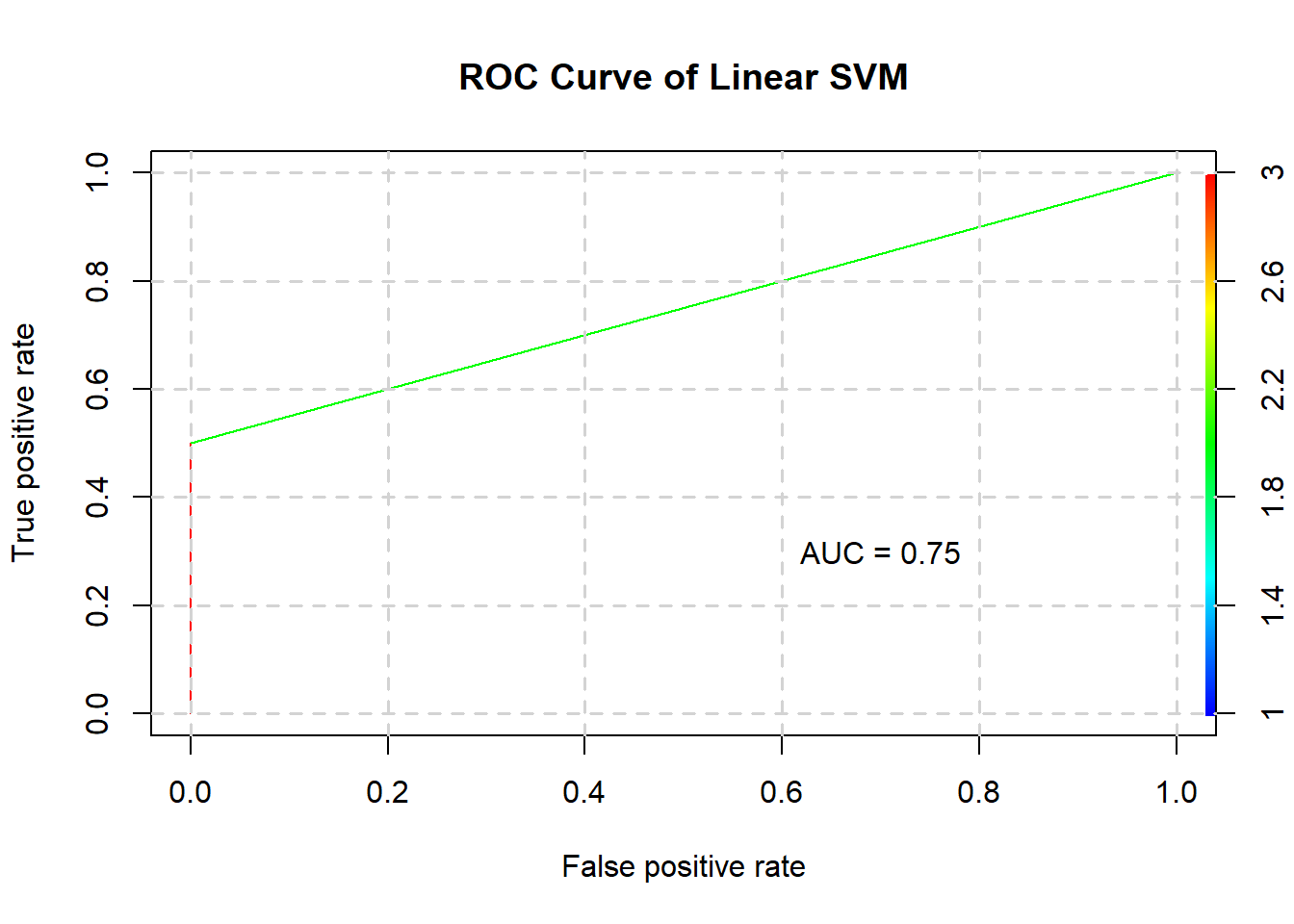

3) Radial support vector machine

radialstats <- confusionMatrix(predict(radialSVM$best.model, testing), testing$Status)
radialstats$byClass

##          Sensitivity          Specificity       Pos Pred Value 
##            0.7500000            1.0000000            1.0000000 
##       Neg Pred Value            Precision               Recall 
##            0.8000000            1.0000000            0.7500000 
##                   F1           Prevalence       Detection Rate 
##            0.8571429            0.5000000            0.3750000 
## Detection Prevalence    Balanced Accuracy 
##            0.3750000            0.8750000

The radial SVM’s confusion matrix is as such:

radialstats$table

##           Reference
## Prediction 1 2
##          1 3 0
##          2 1 4

And its ROC curve and AUC:

plotROC(radialSVM$best.model, testing, "Radial SVM")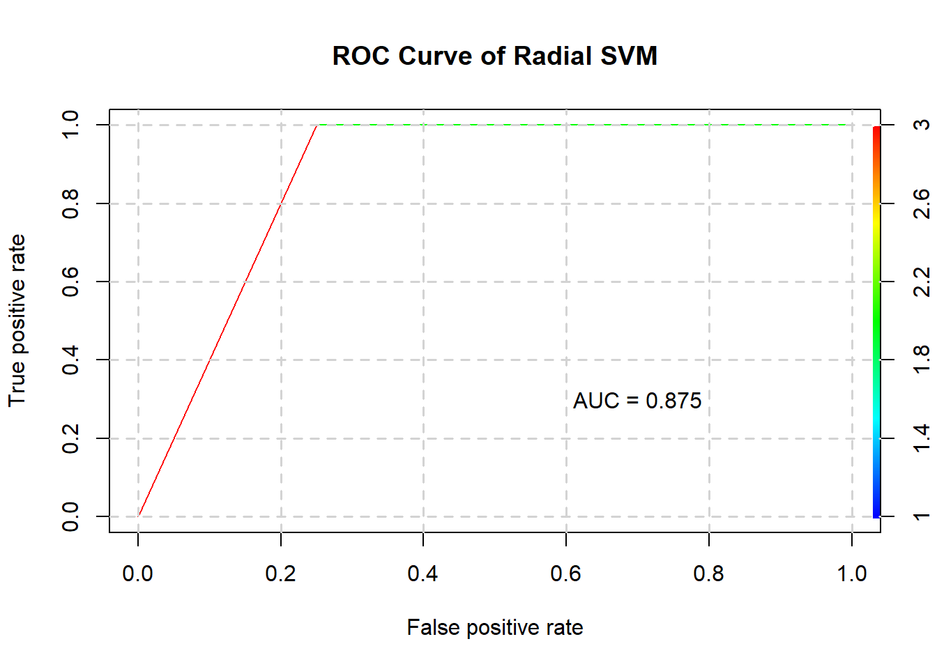

4) Decision tree

rpartstats <- confusionMatrix(predict(rpart, testing), testing$Status)
rpartstats$byClass

##          Sensitivity          Specificity       Pos Pred Value 
##            1.0000000            0.7500000            0.8000000 
##       Neg Pred Value            Precision               Recall 
##            1.0000000            0.8000000            1.0000000 
##                   F1           Prevalence       Detection Rate 
##            0.8888889            0.5000000            0.5000000 
## Detection Prevalence    Balanced Accuracy 
##            0.6250000            0.8750000

The decision tree’s confusion matrix is as such:

rpartstats$table

##           Reference
## Prediction 1 2
##          1 4 1
##          2 0 3

And its ROC curve and AUC:

plotROC(rpart, testing, "Decision Tree")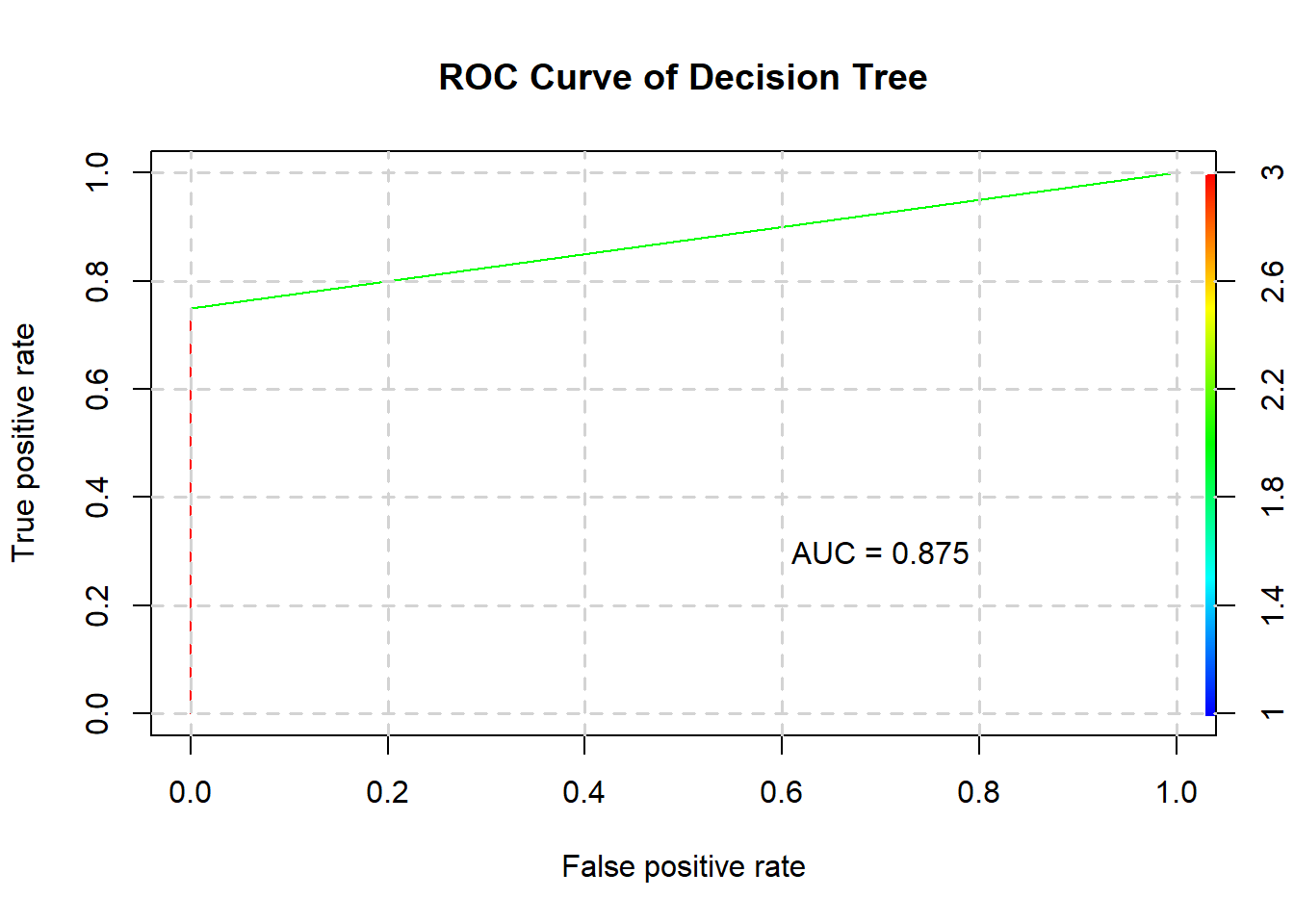

5) Ranger random forest

rangerstats <- confusionMatrix(predict(ranger, testing), testing$Status)
rangerstats$byClass

##          Sensitivity          Specificity       Pos Pred Value 
##            1.0000000            0.7500000            0.8000000 
##       Neg Pred Value            Precision               Recall 
##            1.0000000            0.8000000            1.0000000 
##                   F1           Prevalence       Detection Rate 
##            0.8888889            0.5000000            0.5000000 
## Detection Prevalence    Balanced Accuracy 
##            0.6250000            0.8750000

The ranger random forest’s confusion matrix is as such:

rangerstats$table

##           Reference
## Prediction 1 2
##          1 4 1
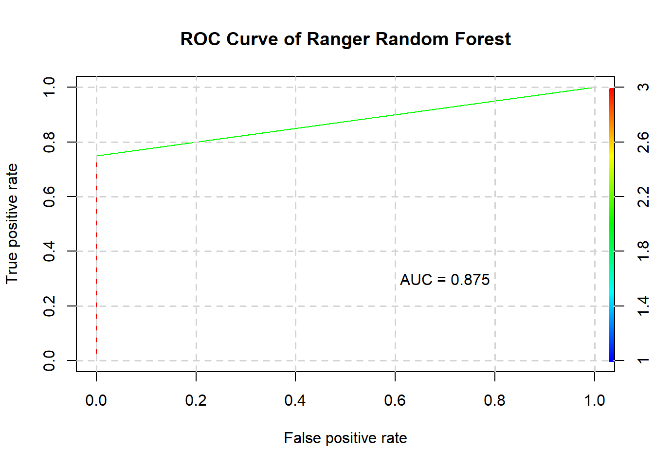
##          2 0 3

And its ROC curve and AUC:

plotROC(ranger, testing, "Ranger Random Forest")

Part 3 My Code

3.1 Setting Up the Working Environment

3.2 Exploring the Data

3.2.1 A heatmap using pheatmap()

3.2.1.1 Performing a little GO-term analysis

3.2.2 Constructing a correlation plot using corrplot()

3.3 Perfoming PCA

3.4 Training the Models

3.4.1 Making the training and testing data

3.4.2 Performing cross validation

3.4.3 Training the models

3.5 Evaluating the Models

3.2.1 A heatmap using `pheatmap()`

3.2.2 Constructing a correlation plot using `corrplot()`