2 Setting up the project.

In Section 2, the setup of the code will be explained including: installing packages, initialising data frames, reading in the dataset, and selecting our parameters.

2.1 Installing the required packages.

Firstly, the following code can be run for a clean installation of the missing packages.

wanted_packages <- c("fBasics", "dplyr", "gtools", "knitr", "boot", "lm.beta", "pROC",
                     "car", "DAAG", "nortest", "MLmetrics", "Metrics", "dLagM", "reticulate")

missing_packages <- wanted_packages[!wanted_packages %in% rownames(installed.packages())]

if (length(missing_packages) > 0) {
    install.packages(missing_packages)
}

lapply(wanted_packages, require, character.only = TRUE)

2.2 Setting up the coding environment.

The purpose of this section is to create some empty variables that we will be utilised within loops, later in the project.

# Setup for the Comparison Table.
Comparison_Table <- data.frame()
# Setup for the Final List.
Final_List <- data.frame()

The required packages for the following code should now be installed!

2.3 Reading the dataset.

The “read.csv” function can be used to import the dataset from a saved .csv file.
A generic file path is given below, be sure to update this in your own code so that it correctly reflects the path to your dataset.

The format of the .csv required should contain, as a minimum, the following column headings:
- “K SETS” (Filled with “1” for building 1, “2” for building 2, … “n” for Building n.)
- “id” (for the university/organisation building number.) - “Building Name” - “Date” of the current reading (dd/mm/yyyy)
- “Days in the Month” for the corresponding date. - “Energy Signature” (Energy consumption in a given month / Hours in said month)
- “Temperature C” (Outdoor average per month)

Each consecutive row of the dataset should then detail the following month’s data.
Each building in the dataset should then have their data appended to the bottom of the dataset.
Below is an example layout.

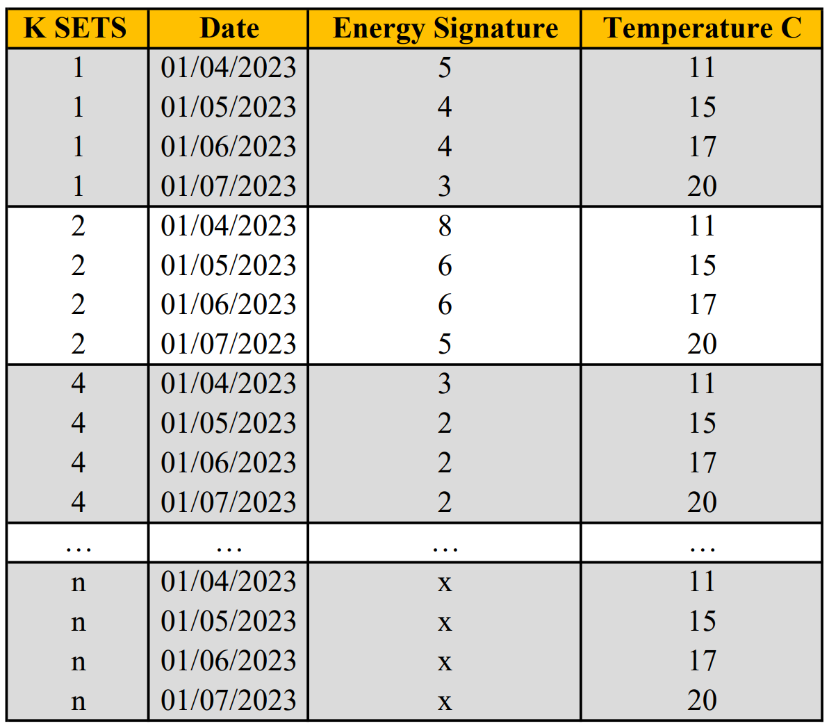
Figure 2.1: A suitable .csv format.

regData <- read.csv("./data/Raw_Data/Example_Data", header = TRUE)

This file can now be readily accessed by calling “regData”.

2.4 Input parameters.

The following chunk is used to input the settings that the code should be run with.
In the dataset assessed here, there were 3 time periods.
Rows 1:32 contained energy readings from the first time period, and therefore “Split_1 <- 1:32”.
The split points of your dataset should be inputted here accordingly.

If there are no splits, the entire dataset should be assessed by “split_1”, i.e.,
“Split_1 <- First_Row:Last_Row”.
If there are more split points, “Split_4”, “Split_5” can be added to the code etc.

– – If the number of split points are altered, don’t forget to edit the “if” conditions in loop 1 – –

#Enter the balance Points to be tested here.
BP_trial <- seq(start_temp, end_temp, by = increment) #E.g. (14, 16, by = 0.5)


# Enter the rows where the csv should be split, and label the Time Periods.
Split_1 <- Row_Start_1:End_1 #E.g. 1:32
Title_1 <- "Time_Period_1"

Split_2 <- Row_Start_2:End_2 #E.g. 33:44
Title_2 <- "Time_Period_2"

Split_3 <- Row_Start_3:End_3 #E.g. 45:60
Title_3 <- "Time_Period_3"