4 Determining the best fitting models.
4.1 Energy Predictions.
The regression analysis conducted returns 3 coefficients for each model created, these can be accessed via the following code,
  # List of Modelling Coefficients.
  Base <- coeffMatrix[1, 1]
  Slope <- coeffMatrix[2, 1]
  Intercept <- coeffMatrix[3, 1]
An energy signature prediction can then be made using the following formula,
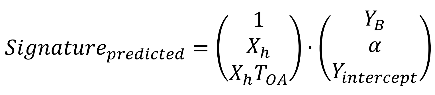
Figure 4.1: Formula for energy predictions
Where YB, \(\alpha\) and Yintercept are the Base, Slope and Intercept coefficients respectively.
This is represented in the code by the following,
  # Energy Signature Prediction.
  Sig_Pred <- Base + (Slope * Dummy_Temp) + (Intercept * Dummy_Variables)
Then by accessing the number of days in each month and multiplying by 24,
the hours per month is obtained.
This can be used with energy signature predictions to create total
consumption predictions.
  # Hours in a given Month.
  Hours_Month <- Current_Set$Days.in.the.Month * 24

  # Energy Prediction.
  Energy_Pred <- Sig_Pred * Hours_Month
Finally, subtracting the predicted consumption away from the measured consumption gives a column of residuals, which will be used to generate the statistical indicators.
  # Calculates the Energy Residuals.
  Residuals <- Energy_Measured - Energy_Pred
4.2 Statistical Indicators.
Well-calibrated building energy models should meet guidelines for at least 4 different statistical indicators, namely Root Mean Square Error [RMSE], Coefficient of variation of RMSE [CV(RMSE)], Coefficient of determination [R2] and Normalised mean bias error [NMBE].
Variance can be calculated with a base R function, the statistical indicators are then calculated with the following formulae,
  # Variance (Sample).
  Var <- var(Energy_Measured)

  # Calculating RMSE, (the 3 represents the degrees of freedom).
  RMSE <- (sum(Residuals^2) / (nTrain - 3))^0.5

  # Coefficient of Variation of Root Mean Square Error.
  CV_RMSE <- 100 * (nTrain * RMSE) / sum(Energy_Measured)

  # Coefficient of Determination R^2.
  R2 <- 100 * (1 - ((sum(Residuals^2)) / (nTrain * Var)))

  # Normalised mean bias error (NMBE).
  NMBE <- 100 * ((sum(Residuals) * nTrain) / ((nTrain - 3) * sum(Energy_Measured)))
4.3 Storing the best-fitting models.
Finally, to conclude this section the best fitting balance point temperatures need
to be isolated.
This is completed in three steps:
1. Add the current data to a comparison table and remove the dummy variables
before the next temperature loop begins.
2. After the temperature loop has been completed, identify the row of data with the
best statistical indicators (in this case RMSE was used).
3. Insert the best model into a new list.
  # Saves data in Comparison_Table for each Balance_Point.
  Comparison_Table[j, 1:10] <- c(
    Current_Set$id[j], Current_Set$Building.Name[j], Balance_Point,
    Base, Intercept, Slope, RMSE, CV_RMSE, R2, NMBE)

  # Removes the Dummy columns before the next loop.
  Current_Set <- Current_Set[, -13:-14]

} # End of Temperature Looping

# Identify the minimum RMSE.
n <- which.min(Comparison_Table$V7)

# Selecting the best fitting values from the Comparison Table and store them in a Final List.
Best_Model_List[i, 1:10] <- Comparison_Table[n, c("V1", "V2", "V3", "V4", "V5",
                                                  "V6", "V7", "V8", "V9", "V10")]