3 Creating the Energy Models.

3.1 Determining the number of loops.

Prior to beginning the first loop, “regData” can be analysed with the following code. This will eventually be used to tell the code in the following sections how many iterations to do.

# number of rows in the csv.
nData <- nrow(regData)

# Arranging k separate sets for the 48 separate buildings.
rowNumbers <- 1:nData
kSets <- max(na.omit(regData$K.SETS))

# Number of Balance points that need to be trialed.
nBP <- length(BP_trial)

3.2 Starting the Time Period Loop.

The chunk of code seen below is used to assign a split in the dataset so that energy models from each time period can be assessed separately.

Importantly, notice how there is an unmatched set of braces “{}”, this is because all of the code in sections 3.3 and 3.4 need to be contained and should be indented within this first loop.

for (x in 1:3) { # Loop 3 times, because there are 3 Time Periods in the example.
    if (x == 1) {
        Current_Rows <- Split_1
        Period <- Title_1}
    if (x == 2) {
        Current_Rows <- Split_2
        Period <- Title_2}
    if (x == 3) {
        Current_Rows <- Split_3
        Period <- Title_3}

The “Current_Rows” will then be used in the following section to separate the relevant data.
The strings saved in “Period”, are used for plotting at the end of the building loop.

3.3 Seperating the Buildings for Looping.

A loop through all of the “K” sets can now be conducted, i.e., to create models for each building separately.
First, we sort the relevant data so that only the current building “i” is modeled. This can be achieved with the lines starting “trainSet” and “trainData”.
“Current_Set” further filters the data by the Time Period currently being looped.
“nTrain” is a variable that will be used later in the project. Similarly, to the previous code chunk, the following code has another open brace, this is because all of the next loop should be indented within this loop too.

 # For each building 'i' in the dataset.
    for (i in 1:kSets) {
        # -------- Data selection --------

        # Select the set rows which correspond to the current building 'i'.
        trainSet <- subset(rowNumbers, regData$K.SETS == i)

        # Selects the data from the csv for modelling, according to the training rows.
        trainData <- regData[trainSet, ]
        
        # Select the correct years of data only.
        Current_Set <- trainData[Current_Rows, ]
        
        # Length of the Current set.
        nTrain <- length(Current_Set)

3.4 Balance Point Testing.

At this stage of the code, we have isolated all of the relevant data and are ready to start creating the building energy models.

Explained as simply as possible, to create “3PH Heating models”, energy signatures will be regressed against a “dummy variable” and a list of the temperatures below the balance point.

The figure below showcases the logic to select dummy variables.
Where T_OA is the outdoor air temperature, T_BP is the balance point temperature, and X_h is the dummy variable,

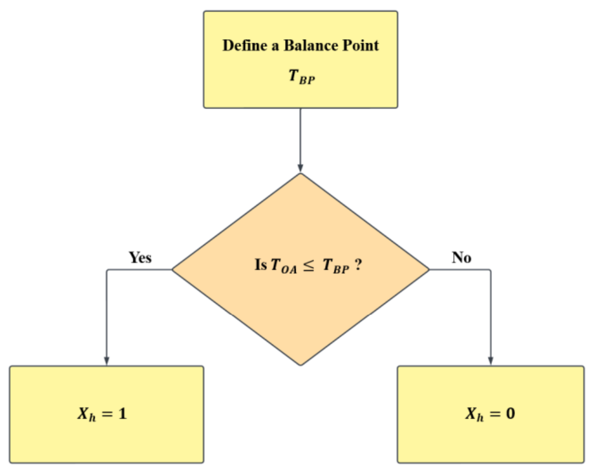
Figure 3.1: Dummy variable logic.

One final loop is created to test each potential “Balance Point”. For each, the dummy variables are created using the recorded temperatures.
A list of the temperatures below the balance point can simply be created by multiplying the Temperatures and the Dummy Variables.
Finally, these new columns are binded to the “Current_Set” of data.

        # For each Balance Point 'j' that we are testing.
        for (j in 1:nBP) {
            # -------- Dummy Variables --------
            # Selects the temperature column.
            Temperatures <- Current_Set$Temperature.C

            # Assigns the current Balance Point that needs to be tested.
            Balance_Point <- BP_trial[j]

            # Compares values against the Balance point.
            # If a value is below the balance point, returns a 1,
            # Else, returns a 0.
            Dummy_Variables <- ifelse(Temperatures <= Balance_Point, 1, 0)

            # Creates the "modified temperature list", i.e., the temperature list with
            # zeros in place of temperatures greater than the balance point.
            Dummy_Temp <- Temperatures * Dummy_Variables

            # Adds the Dummy Variables and Dummy*Temp list from the current Balance Point
            # to this the Training Data set.
            Current_Set <- cbind(Current_Set, Dummy_Variables, Dummy_Temp)

3.5 Regression Analysis.

Finally, to end this section of the project, the regression models will be created.
These can simply be created using the linear model “lm” function.
The regression coefficients are then saved into the coefficient matrix.

  # Creates the linear Regression models.
  regModel <- lm(Energy.Signature ~ Dummy_Temp + Dummy_Variables, data = Current_Set)

  # Creating the Coefficient Matrix.
  coeffMatrix <- cbind(summary.lm(regModel)$coefficients)