Part 5 Week 3

Getting Started with Data Visualization in R > Week 3

5.1 Creating reports with R Markdown

install.packages("tinytex")
tinytex::install_tinytex()

5.1.1 R Markdown

This is an R Markdown document. Markdown is a simple formatting syntax for authoring HTML, PDF, and MS Word documents. For more details on using R Markdown see http://rmarkdown.rstudio.com.

When you click the Knit button a document will be generated that includes both content as well as the output of any embedded R code chunks within the document. You can embed an R code chunk like this:

summary(cars)

#>      speed           dist    
#>  Min.   : 4.0   Min.   :  2  
#>  1st Qu.:12.0   1st Qu.: 26  
#>  Median :15.0   Median : 36  
#>  Mean   :15.4   Mean   : 43  
#>  3rd Qu.:19.0   3rd Qu.: 56  
#>  Max.   :25.0   Max.   :120

5.1.2 Including Plots

You can also embed plots, for example:

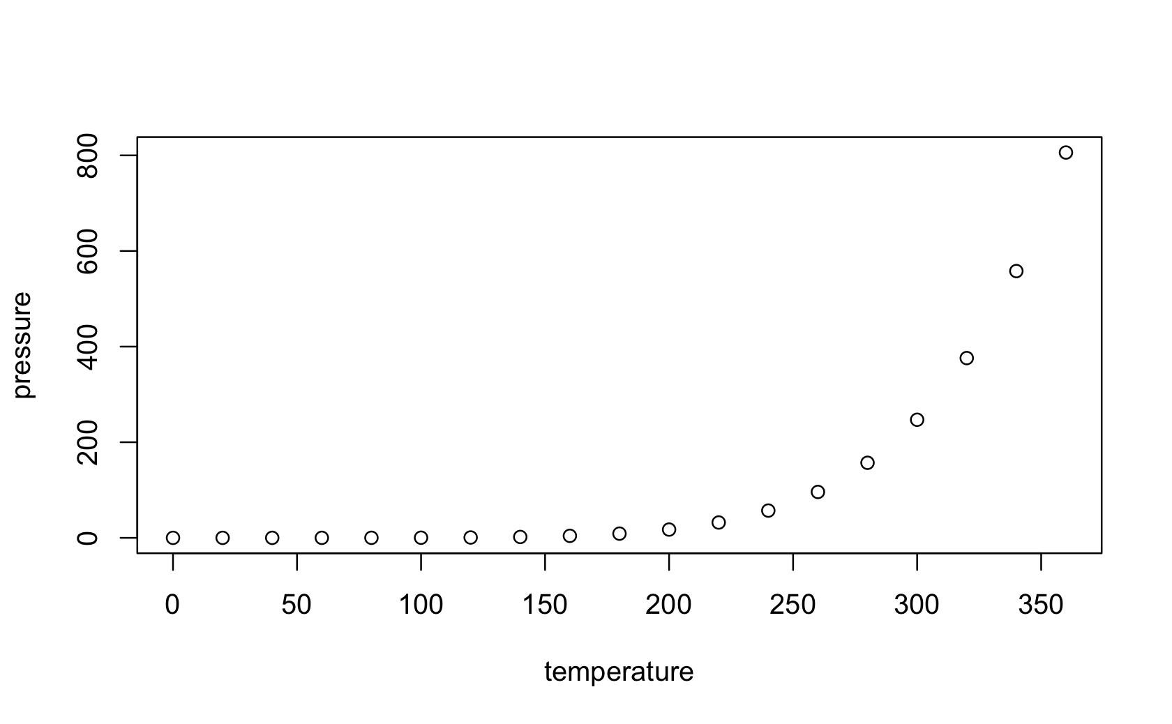
Note that the echo = FALSE parameter was added to the code chunk to prevent printing of the R code that generated the plot.

5.2 R Markdown Cheat Sheet

https://www.rstudio.com/wp-content/uploads/2015/02/rmarkdown-cheatsheet.pdf

5.3 R Markdown syntax and tables

This is just normal written text in an RMarkdown file. There ’s nothing special about this. This is normal paragraph text.

You can start a new paragraph just by hitting enter and putting in a blank line.

If you want text in italics or bold you need to mark that with either *one* or **two** asterisks on either side.

If you want text to like verbatim code you should surround it with one backtick on both sides.

You can do superscripts¹ surrounding text with carets (^) or subscripts₁ by surrounding texts with tildes (~).

Endashs – are two minus signs, emdashes — are three minus signs.

A block quote is preceded by a greater than sign. A block quote is preceded by a greater than sign. A block quote is preceded by a greater than sign. A block quote is preceded by a greater than sign. A block quote is preceded by a greater than sign.

# Different Levels of Header
## Are preceded with increasing
### Numbers of pound signs (hashtags#)

You can make bullet lists. Put a blank line after paragraph graph text. Then, on the next like, use an asterisks (*) for the top bullet. For sub-items, on a new line, press tab and then use a plus sign (+). For sub-sub items, press tab twice and use a minus sign (-)

My bullets
- sub-item 1
  - sub-sub-item 1

For numbered lists, start the number list item with a number followed by a period (1.)

Number 1
Number 2

Right	Left	Default	Center
You	can	make	a
table	by	hand	but
it	is	clunky	.

To see more formatting options, look at the second page of the RMarkdown cheatsheet.

For a really, really detailed look at R Markdown, see the Definitive Guide by Xie, Allaire, and Grolemund

5.4 qplots and closing thoughts

# knitr::opts_chunk$set(echo = TRUE)

library(tidyverse)
library(knitr)

# setwd("week3")

dat <- read_csv("cces_sample_coursera.csv")

#> 
#> ── Column specification ──────────────────────────────────────────────────────────────────────────────────
#> cols(
#>   .default = col_double()
#> )
#> ℹ Use `spec()` for the full column specifications.

dat <- drop_na(dat)

5.4.1 My first tables

kable(table(dat$gender), align = "l")

Var1	Freq
1	391
2	478

#?kable
kable(summarise(
  dat,
  Mean = mean(dat$faminc_new),
  Median = median(dat$faminc_new)
),
align = "l",
label = "Summary Statistics for Family Income")

Mean	Median
6.581	6

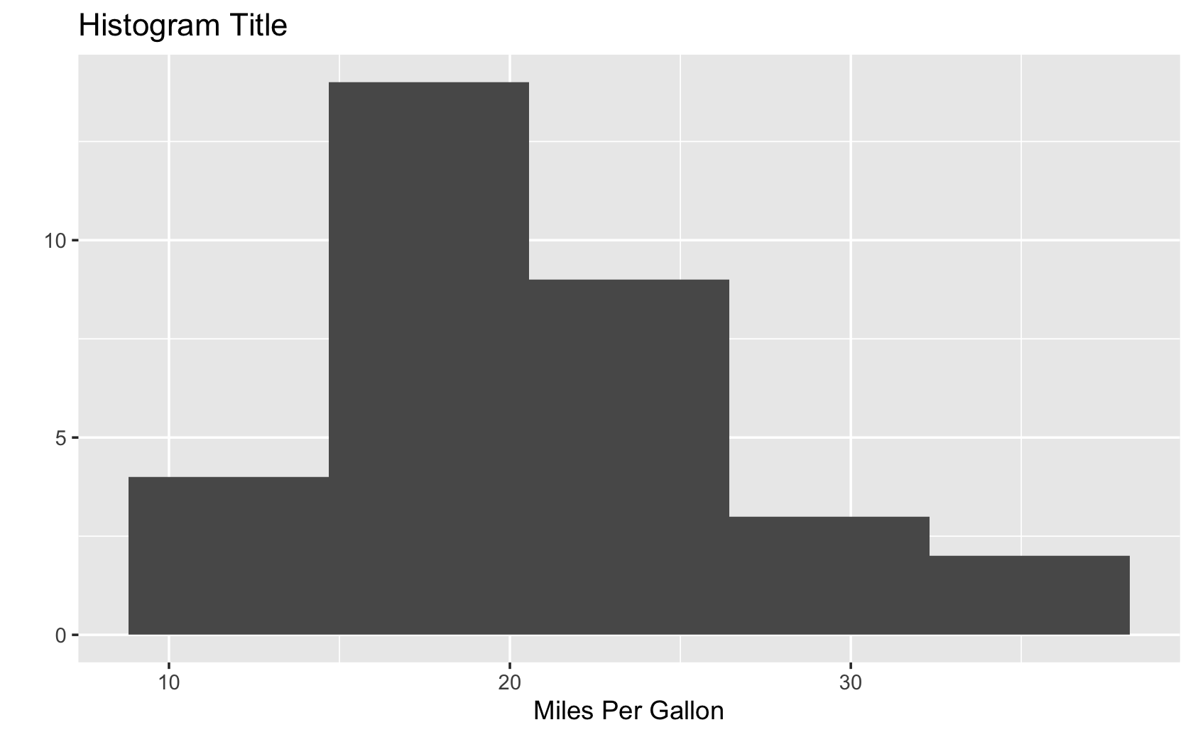
5.4.2 My first QPlots

These examples inspired by UC Business Analytics R Programming Guide.

See also the documentation page for qplot., which you can also access with ?qplot in the R console.

data(mtcars)

qplot(
  x = mpg,
  data = mtcars,
  geom = "histogram",
  bins = 5,
  main = "Histogram Title",
  xlab = "Miles Per Gallon"
)

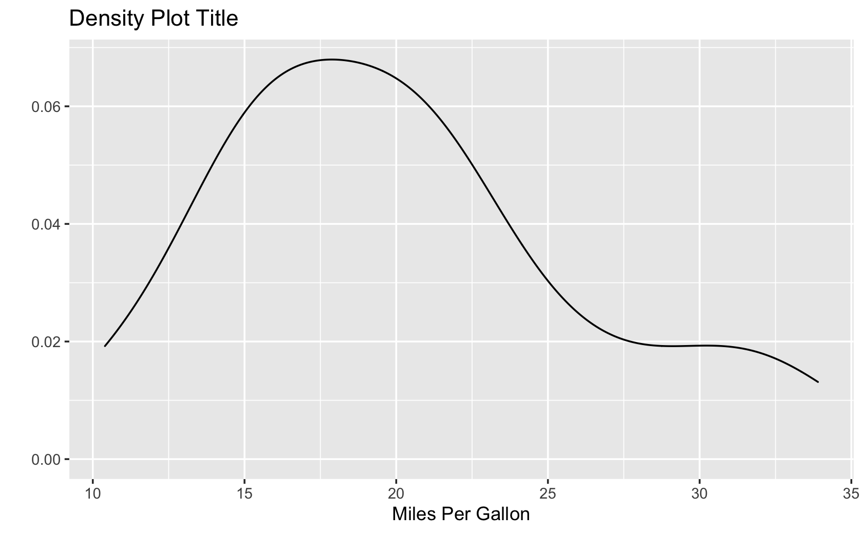
qplot(
  x = mpg,
  data = mtcars,
  geom = "density",
  main = "Density Plot Title",
  xlab = "Miles Per Gallon"
)

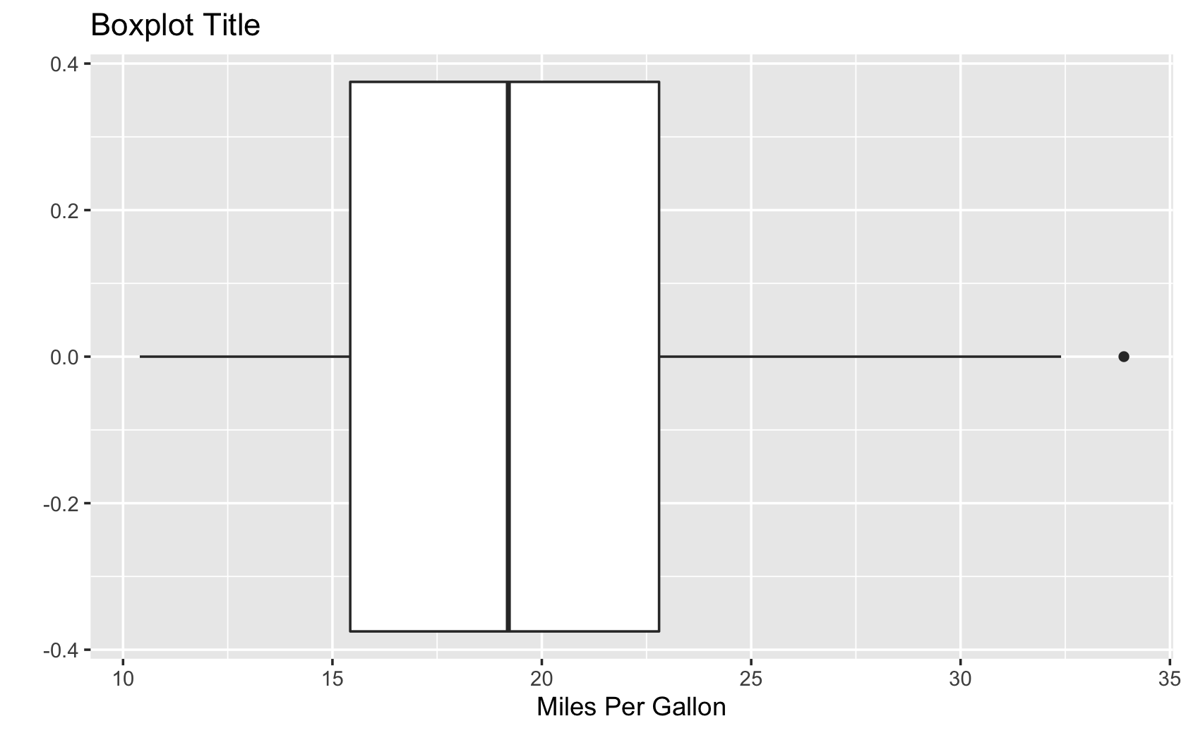
qplot(
  x = mpg,
  data = mtcars,
  geom = "boxplot",
  main = "Boxplot Title",
  xlab = "Miles Per Gallon"
)

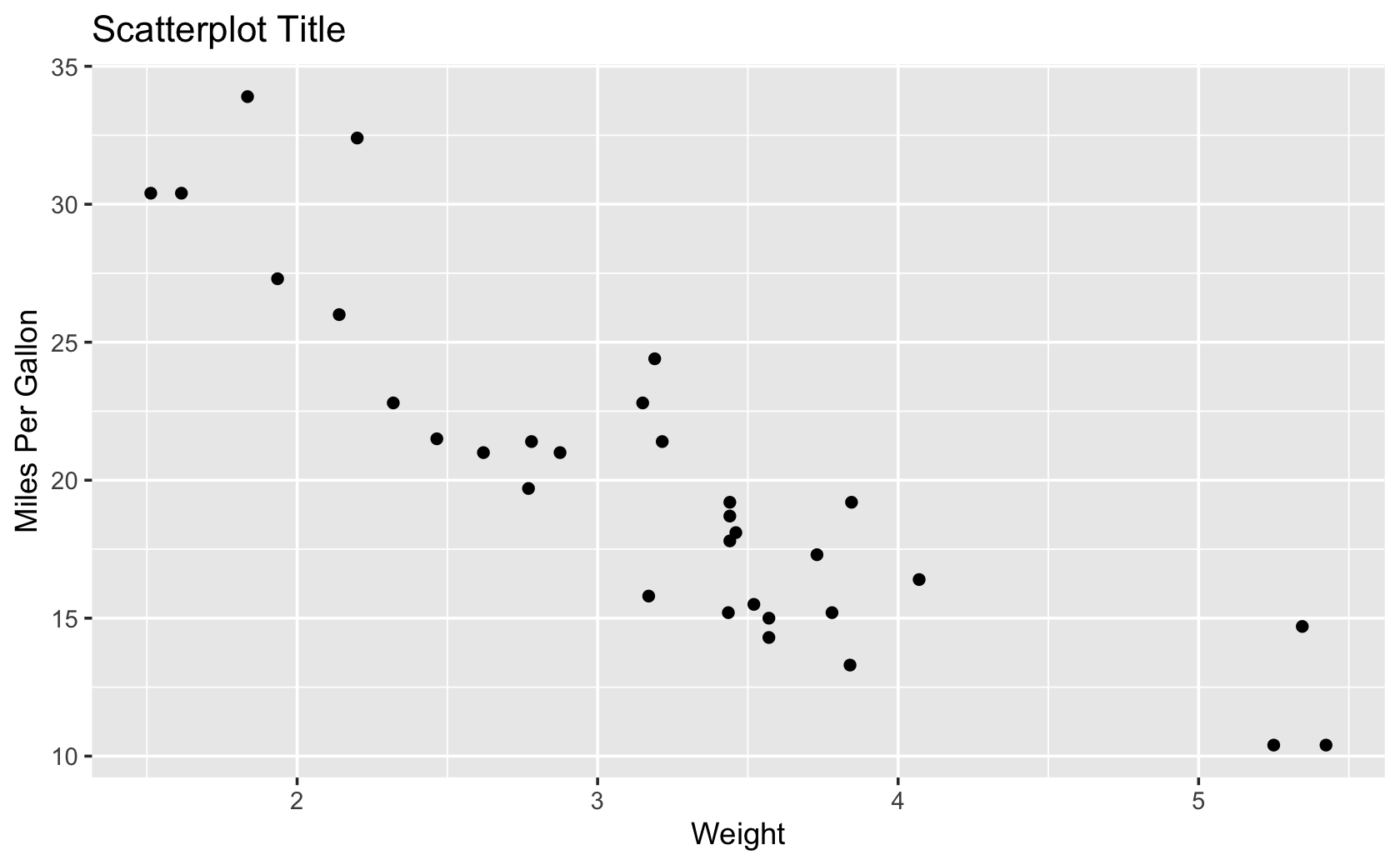
qplot(
  x = wt,
  y = mpg,
  data = mtcars,
  geom = "point",
  main = "Scatterplot Title",
  xlab = "Weight",
  ylab = "Miles Per Gallon"
)

5.5 Practices

5.5.1 Problem 1

Create a vector of five numbers of your choice between 0 and 10, save that vector to an object, and use the sum() function to calculate the sum of the numbers.

a <- c(1, 3, 5, 7, 9)
sum(a)

#> [1] 25

5.5.2 Problem 2

Create a data frame that includes two columns. One column must have the numbers 1 through 5, and the other column must have the numbers 6 through 10. The first column must be named “alpha” and the second column must be named “beta.” Name the object “my_dat.” Display the data.

Put your code and solution here:

alpha <- 1:5
beta <- 6:10
my_dat <- data.frame(alpha, beta)
my_dat

#>   alpha beta
#> 1     1    6
#> 2     2    7
#> 3     3    8
#> 4     4    9
#> 5     5   10

5.5.3 Problem 3

Using the data frame created in Problem 2, use the summary() command a create a five-number summary for the column named “beta.”

Put your code and solution here:

summary(my_dat$beta)

#>    Min. 1st Qu.  Median    Mean 3rd Qu.    Max. 
#>       6       7       8       8       9      10

5.5.4 Problem 4

There is code for importing the example survey data that will run automatically in the setup chunk for this report (Line 13). Using that data, make a boxplot of the Family Income column using the Base R function (not a figure drawn using qplot). Include your name in the title for the plot. Your name should be in the title. Relabel that x-axis as “Family Income.”

Hint: consult the codebook to identify the correct column name for the family income question.

Put your code and solution here:

boxplot(dat$faminc_new, 
        main = "Haoqi's Boxplot of Family Income",
        xlab = "Family Income")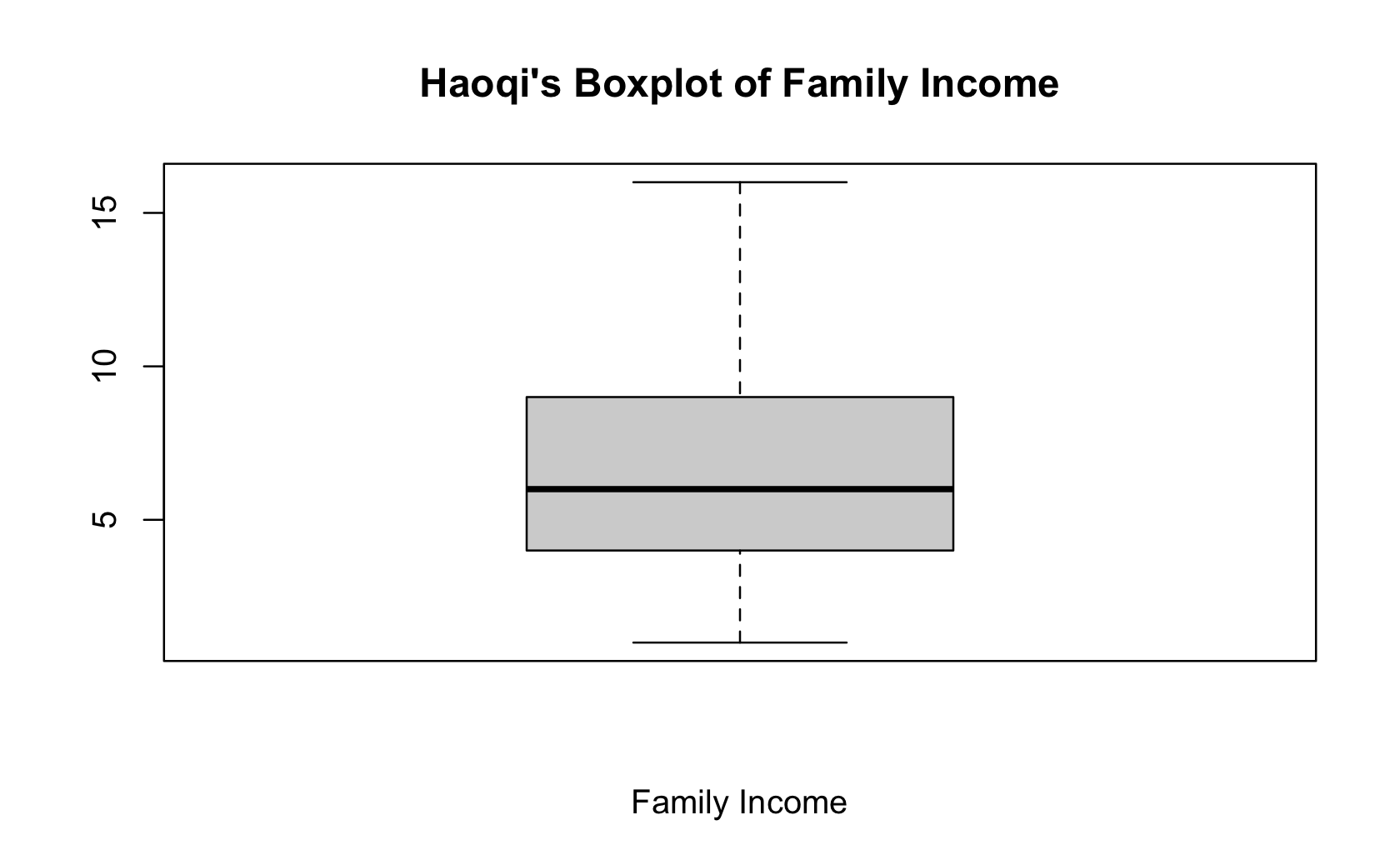

5.5.5 Problem 5

Using the survey data, filter to subset the survey data so you only have male survey respondents who live in the northwest or midwest of the United States, are married, and identify as being interested in the news most of the time.

Use the str() function to provide information about the resulting dataset.

Put your code and solution here:

dat %>% glimpse()

#> Rows: 869
#> Columns: 25
#> $ caseid       <int> 417614315, 415490556, 414351505, 411855339, 420208067, 412517331, 412873566, 412948037, 415732…
#> $ region       <int> 3, 1, 3, 1, 2, 1, 2, 1, 3, 3, 1, 3, 4, 3, 2, 4, 2, 3, 1, 1, 4, 4, 3, 3, 1, 4, 3, 3, 1, 4, 2, 3…
#> $ gender       <int> 1, 2, 2, 2, 1, 1, 2, 1, 1, 2, 2, 1, 1, 2, 2, 1, 2, 2, 1, 1, 1, 2, 2, 1, 1, 2, 1, 1, 2, 1, 2, 1…
#> $ educ         <int> 2, 6, 3, 5, 3, 2, 3, 5, 6, 2, 3, 6, 3, 3, 6, 3, 4, 4, 6, 5, 6, 3, 6, 5, 5, 2, 5, 6, 5, 6, 5, 2…
#> $ edloan       <int> 2, 2, 2, 2, 2, 2, 2, 1, 2, 2, 2, 2, 2, 1, 1, 2, 2, 2, 2, 2, 2, 2, 1, 2, 1, 2, 2, 2, 1, 1, 2, 2…
#> $ race         <int> 1, 1, 2, 6, 1, 1, 1, 1, 1, 1, 1, 1, 3, 2, 1, 1, 1, 1, 1, 1, 1, 1, 1, 1, 1, 3, 1, 1, 2, 1, 1, 1…
#> $ hispanic     <int> 2, 1, 2, 2, 2, 2, 2, 2, 2, 2, 2, 2, 2, 2, 2, 2, 2, 2, 2, 2, 2, 2, 2, 2, 2, 2, 2, 2, 2, 2, 2, 2…
#> $ employ       <int> 5, 1, 1, 5, 1, 5, 7, 1, 1, 5, 7, 1, 4, 1, 9, 1, 4, 6, 1, 3, 1, 1, 1, 6, 1, 9, 5, 5, 4, 1, 6, 1…
#> $ marstat      <int> 3, 1, 4, 3, 1, 5, 1, 1, 5, 4, 1, 1, 5, 2, 1, 5, 5, 3, 1, 5, 1, 5, 1, 5, 1, 5, 1, 1, 1, 1, 5, 1…
#> $ pid7         <int> 6, 2, 2, 3, 4, 5, 7, 1, 6, 5, 3, 6, 1, 1, 2, 2, 3, 7, 4, 3, 6, 5, 7, 2, 4, 1, 4, 1, 1, 6, 1, 3…
#> $ ideo5        <int> 3, 2, 3, 1, 5, 4, 5, 1, 5, 3, 3, 5, 1, 3, 1, 1, 1, 3, 3, 1, 3, 4, 5, 1, 3, 3, 4, 2, 2, 4, 1, 3…
#> $ pew_religimp <int> 1, 3, 1, 2, 4, 3, 1, 4, 4, 1, 2, 1, 3, 2, 2, 4, 4, 1, 4, 4, 3, 3, 1, 4, 1, 3, 2, 3, 4, 1, 4, 4…
#> $ newsint      <int> 2, 3, 3, 1, 1, 2, 3, 1, 4, 1, 1, 1, 2, 3, 1, 1, 3, 1, 1, 1, 1, 2, 1, 4, 1, 1, 1, 1, 1, 1, 2, 2…
#> $ faminc_new   <int> 1, 12, 4, 6, 10, 6, 2, 11, 16, 4, 11, 11, 1, 3, 11, 9, 2, 3, 10, 8, 12, 6, 11, 6, 9, 4, 10, 11…
#> $ union        <int> 3, 3, 3, 2, 1, 3, 3, 2, 3, 3, 3, 3, 3, 2, 3, 3, 3, 2, 3, 3, 3, 3, 3, 3, 3, 1, 3, 2, 3, 3, 3, 3…
#> $ investor     <int> 2, 2, 1, 1, 2, 1, 2, 1, 2, 2, 1, 1, 2, 1, 1, 1, 2, 2, 1, 2, 2, 2, 1, 1, 1, 2, 1, 1, 2, 1, 2, 1…
#> $ CC18_308a    <int> 2, 4, 4, 4, 4, 1, 1, 4, 1, 4, 4, 1, 4, 4, 4, 4, 4, 1, 4, 4, 2, 2, 1, 4, 1, 4, 1, 4, 4, 2, 4, 4…
#> $ CC18_310a    <int> 2, 3, 2, 3, 2, 3, 2, 3, 2, 2, 3, 2, 1, 3, 5, 3, 2, 2, 3, 2, 2, 3, 2, 2, 3, 3, 3, 2, 3, 2, 3, 2…
#> $ CC18_310b    <int> 3, 2, 2, 3, 2, 3, 2, 3, 3, 3, 3, 2, 1, 5, 3, 3, 5, 3, 3, 3, 2, 3, 2, 2, 3, 3, 3, 3, 3, 2, 3, 2…
#> $ CC18_310c    <int> 3, 5, 2, 3, 3, 2, 3, 3, 2, 2, 3, 2, 1, 2, 2, 3, 3, 2, 3, 3, 2, 3, 2, 2, 3, 3, 3, 2, 3, 2, 3, 2…
#> $ CC18_310d    <int> 5, 5, 2, 3, 2, 2, 5, 5, 5, 5, 3, 2, 3, 5, 3, 3, 2, 2, 3, 3, 3, 3, 2, 3, 3, 5, 2, 2, 3, 3, 3, 2…
#> $ CC18_325a    <int> 1, 2, 1, 2, 1, 1, 1, 2, 2, 2, 2, 1, 2, 2, 2, 2, 2, 2, 1, 2, 1, 1, 1, 2, 1, 2, 1, 2, 1, 1, 2, 2…
#> $ CC18_325b    <int> 2, 2, 2, 1, 2, 1, 1, 2, 1, 1, 1, 1, 1, 2, 1, 1, 1, 2, 1, 1, 1, 1, 2, 1, 1, 1, 1, 1, 2, 1, 1, 1…
#> $ CC18_325c    <int> 1, 2, 1, 2, 1, 1, 1, 2, 1, 2, 2, 1, 2, 2, 2, 1, 2, 1, 2, 2, 1, 2, 2, 2, 1, 2, 1, 2, 2, 1, 2, 1…
#> $ CC18_325d    <int> 1, 1, 2, 1, 1, 1, 1, 1, 2, 1, 2, 1, 2, 1, 2, 1, 1, 1, 1, 1, 1, 2, 2, 1, 1, 1, 1, 1, 2, 1, 1, 1…

# male: gender == 1
# northwest or midwest: region %in% c(1, 2)
# married: marstat == 1
# interested in the news most of the time: newsint == 1

dat %>% 
  filter(gender == 1 & region %in% c(1, 2) & marstat == 1 & newsint == 1) %>% 
  str()

#> 'data.frame':    75 obs. of  25 variables:
#>  $ caseid      : int  420208067 412948037 411855595 414480371 416806180 414729651 412021973 412348831 412929385 412047867 ...
#>  $ region      : int  2 1 1 1 2 2 1 2 1 2 ...
#>  $ gender      : int  1 1 1 1 1 1 1 1 1 1 ...
#>  $ educ        : int  3 5 6 5 3 2 6 5 5 5 ...
#>  $ edloan      : int  2 1 2 1 1 2 2 2 2 2 ...
#>  $ race        : int  1 1 1 1 1 1 1 1 1 1 ...
#>  $ hispanic    : int  2 2 2 2 2 2 2 2 2 2 ...
#>  $ employ      : int  1 1 1 1 1 5 5 1 1 1 ...
#>  $ marstat     : int  1 1 1 1 1 1 1 1 1 1 ...
#>  $ pid7        : int  4 1 4 4 6 2 1 1 1 7 ...
#>  $ ideo5       : int  5 1 3 3 3 1 2 3 1 5 ...
#>  $ pew_religimp: int  4 4 4 1 2 4 4 2 4 1 ...
#>  $ newsint     : int  1 1 1 1 1 1 1 1 1 1 ...
#>  $ faminc_new  : int  10 11 10 9 10 2 13 8 7 11 ...
#>  $ union       : int  1 2 3 3 1 3 2 2 2 3 ...
#>  $ investor    : int  2 1 1 1 1 2 1 2 1 2 ...
#>  $ CC18_308a   : int  4 4 4 1 2 3 4 4 4 1 ...
#>  $ CC18_310a   : int  2 3 3 3 2 2 3 2 3 2 ...
#>  $ CC18_310b   : int  2 3 3 3 2 3 3 5 3 3 ...
#>  $ CC18_310c   : int  3 3 3 3 3 3 2 5 3 3 ...
#>  $ CC18_310d   : int  2 5 3 3 3 2 2 2 3 3 ...
#>  $ CC18_325a   : int  1 2 1 1 1 2 2 2 2 1 ...
#>  $ CC18_325b   : int  2 2 1 1 1 1 2 1 2 2 ...
#>  $ CC18_325c   : int  1 2 2 1 1 2 2 1 2 2 ...
#>  $ CC18_325d   : int  1 1 1 1 1 1 1 1 2 1 ...

5.5.6 Problem 6

Filter the data the same as in Problem 5. Use a R function to create a frequency table for the responses for the question asking whether these survey respondents are invested in the stock market.

Put your code and solution here:

dat %>% 
  filter(gender == 1 & region %in% c(1, 2) & marstat == 1 & newsint == 1) %>% 
  count(investor)

#>   investor  n
#> 1        1 57
#> 2        2 18

5.5.7 Problem 7

Going back to using all rows in the dataset, create a new column in the data using mutate that is equal to either 0, 1, or 2, to reflect whether the respondent supports increasing the standard deduction from 12,000 to 25,000, supports cutting the corporate income tax rate from 39 to 21 percent, or both. Name the column “tax_scale.” Hint: you’ll need to use recode() as well.

Display the first twenty elements of the new column you create.

Put your code and solution here:

# 0: If the respondent supports neither of the two initiatives
# CC18_325d == 2 & CC18_325a == 2
# 1: If the respondent supports either of the two initiatives
# (CC18_325a == 1 & CC18_325d == 2) | (CC18_325a == 2 & CC18_325d == 1)
# 2: If the respondent supports both initiatives
# CC18_325d == 1 & CC18_325a == 1

dat %>% 
  mutate(tax_scale = case_when(
    (CC18_325d == 2 & CC18_325a == 2) ~ 0,
    ((CC18_325a == 1 & CC18_325d == 2) | (CC18_325a == 2 & CC18_325d == 1)) ~ 1,
    (CC18_325d == 1 & CC18_325a == 1) ~ 2
  )) %>% 
  select(tax_scale) %>% 
  pull() %>% 
  .[1:20]

#>  [1] 2 1 1 1 2 2 2 1 0 1 0 2 0 1 0 1 1 1 2 1

5.5.8 Problem 8

Use a frequency table command to show how many 0s, 1s, and 2s are in the column you created in Problem 7.

Put your code and solution here:

dat %>% 
  mutate(tax_scale = case_when(
    (CC18_325d == 2 & CC18_325a == 2) ~ 0,
    ((CC18_325a == 1 & CC18_325d == 2) | (CC18_325a == 2 & CC18_325d == 1)) ~ 1,
    (CC18_325d == 1 & CC18_325a == 1) ~ 2
  )) %>% 
  select(tax_scale) %>% 
  table()

#> .
#>   0   1   2 
#> 130 408 331

5.5.9 Problem 9

Again using all rows in the original dataset, use summarise and group_by to calculate the average (mean) job of approval for President Trump in each of the four regions listed in the “region” column.

Put your code and solution here:

dat %>% 
  group_by(region) %>% 
  summarise(Trump_Approve_Mean = mean(CC18_308a))

#> # A tibble: 4 x 2
#>   region Trump_Approve_Mean
#>    <int>              <dbl>
#> 1      1               2.77
#> 2      2               2.76
#> 3      3               2.71
#> 4      4               3.03

5.5.10 Problem 10

Again start with all rows in the original dataset, use summarise() to create a summary table for survey respondents who are not investors and who have an annual family income of between $40,000 and $119,999 per year. The table should have the mean, median and standard deviations for the importance of religion column.

Put your code and solution here:

# respondents who are not investors and who have an annual family income of between $40,000 and $119,999 per year
# investor == 2 & faminc_new %in% c(5:10)

dat %>% 
  filter(investor == 2 & (faminc_new %in% c(5:10))) %>% 
  summarise(`Mean Religion Imp.` = mean(pew_religimp),
            ` Median Religion Imp.` = median(pew_religimp),
            ` Standard Dev. Religion Imp.` = sd(pew_religimp))

#>   Mean Religion Imp.  Median Religion Imp.  Standard Dev. Religion Imp.
#> 1              2.326                     2                        1.189

dat %>% 
  filter(investor == 2 & (faminc_new %in% c(5:10))) %>% 
  summarise(
    across(pew_religimp, list(Mean = mean, Median = median, SD = sd))
  )

#>   pew_religimp_Mean pew_religimp_Median pew_religimp_SD
#> 1             2.326                   2           1.189

5.5.11 Problem 11

Use kable() and the the summarise() function to create a table with one row and three columns that provides the mean, median, and standard deviation for the column named faminc_new in the survey data.

Put your code and solution here:

dat %>% 
  summarise(
    Mean = mean(faminc_new), 
    Median = median(faminc_new),
    `Std. Dev` = sd(faminc_new)
  ) %>% 
  knitr::kable()

Mean	Median	Std. Dev
6.581	6	3.247

5.5.12 Problem 12

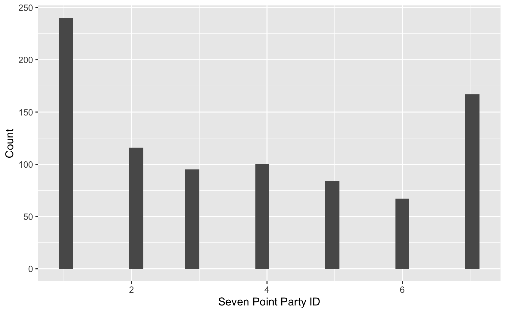
With the survey data, use qplot() to make a histogram of the column named pid7. Change the x-axis label to “Seven Point Party ID” and the y-axis label to “Count.”

Note: you can ignore the “stat_bin()” message that R generates when you draw this. The setup for the code chunk will suppress the message.

Put your code and solution here:

qplot(
  x = pid7,
  data = dat,
  geom = "histogram",
  xlab = "Seven Point Party ID",
  ylab = "Count"
)