Chapter 3 METHODOLOGIES
The surveys were carried out in the autumn of 2021, to collect lithological, structural data and RBF rock samples. Geological data during the field activity were recorded through the Fieldmove app, to be processed later in Qgis. Structural data instead were processed with Tectonics FP to produce stereo plots. Twelve oriented samples from the fault zone were collected to document and analyze the microstructures of the RBF rocks that accommodate the displacement of the roof block. The microstructures described in chapter 5 (microscope observations) are those that appear in the samples. Particular care was taken during the sampling and transport of these rocks from the field to the laboratory to avoid disintegration. Given the fractured and brittle nature of these fault rocks, samples were impregnated and stabilized with epoxy resin. In the following chapter, all the methodologies used for the realization of this thesis work will be described in chronological order.
3.1 Fieldmove App
Global Positioning System (GPS) devices are commonly used to aid navigation, having grown in popularity over the past decade. Over the last few years, this has extended to smartphones and digital compasses, which are often equipped with GPS functionality. GPS is a valuable aid to navigation during fieldwork, although it is important to keep safety at the forefront. Modern technologies are created to facilitate the task. Knowledge of new programs and mastery of functions is the clue to success in any scope. What could be edited only after field nowadays can be partly automatized in the field, processing the information and thus significantly reducing the field period and simplifying the cameral period.
FieldMove is a map-based digital field mapping app for geological data
capture. The app is presented in a map-centric format for use on larger
touchscreen tablets. When sufficient data has been collected, you can
use the drawing tools that include a virtual cursor for precision
drawing to create geological boundaries, fault traces and other linework
on your basemap. It is also possible to create simple polygons to show
the distribution of different rock types. FieldMove relies on three
sensors inside your device, a magnetometer, a gyroscope and an
accelerometer. Together, these sensors can be programmed to measure the
orientation of planar and linear features in the field. All three
sensors are installed as standard in iPhones and iPads, but are not
always present in other hardware devices. You should always check your
device to ensure that all three sensors are present and that the compass and the clinometer give accurate readings before starting
to collect data. You can choose to manually enter data if you do not
trust the internal sensors, or if you are using a traditional hand-held
compass clinometer. FieldMove supports Mapbox™ online maps and can cache
this extensive online map service to work offline in the field. In
addition to handling online maps, geo-referenced basemaps in MBTile or
GeoTIFF format can be imported and also are available offline when
working in the field.
Data can be exported as MOVE, CSV or KMZ files.
3.2 Quantum Gis Software (QGIS)
GIS is the acronym for Geographical Information System, often also
called the Territorial Information System (SIT), an information system
computerized that allows the acquisition, the recording, the analysis,
the visualization and the return of information deriving from
geographical data. It is a capable computer system to produce, manage
and analyze spatial data by associating one or more geographic elements
with each geographic element information. Through a GIS program, the
user is able to view and superimpose different maps themes of a specific
area, ensuring the correspondence of the geographical coordinates of the
scale and, therefore, distances. Themes can be images, for example, aerial
and satellite photos (called raster data) or drawings, e.g. reference
points, contour lines, geological limits (vector files). A GIS stores
the position of data using a projection and coordinate system that
defines the geographic location of the object. The GIS can also manage data from different systems at the same time projection and reference and carry out conversions between the various systems.
Unlike cartography on paper, the scale in a GIS does not indicate the
display scale (in fact in whatever GIS it is the various portions of the
territory can be enlarged as desired) but highlights the quality of
data. Data collected in a GIS system are usually represented through
cartograms or tables relating to more or less extensive areas but,
unlike other computer systems, there are almost infinite possibilities
of use.
In fact, GIS technology integrates 2 systems:
the computerized or CAD design system;
the relational database DBMS or Data Base Management System;
Thus allowing both to carry out the analysis and research operations of Databases, with the geographical analysis and the typical representation of the CAD. In this way there is a greater yield because it is possible to analyze a geographical area at 360 ° by simultaneously analyzing:
Geometric data (shape, size, geographical position of the objects);
Topological data (connection, adjacency and reciprocal relations between objects);
Information data (numerical or textual data relating to objects)
In this way, it is possible to simultaneously analyze a geographical entity under different aspects in a more interactive, effective, and immediate way. QuantumGIS (QGIS) (www.qgis.org) is an Open Source GIS software (it is, therefore, possible to copy and distribute it in perfect legality) that allows you to view, query, modify cards, create, print and perform simple spatial analyzes. QGIS, used as an interface to the most powerful software GIS Open Source GRASS (http://grass.osgeo.org), allows you to create the most different and complex geographic analysis operations such as spatial modeling and image analysis satellite. The main advantages of QGIS are the fact of being free software, having a user-friendly interface, allowing easy analysis of spatial data, and presenting an architecture that can be adapted to different functions thanks to the use of specific plugins. One of its main capabilities is to allow users to view and overlay vector and raster data in different projections and formats without the need to convert them to internal or common files.
3.3 Tectonics FP
TectonicsFP for WindowsTM operating systems is a menu–driven computer program that can produce stereographic plots of orientation data (great circles, poles, lineations). Frequently used statistical procedures like calculating eigenvalues and eigenvectors, calculating mean vector with concentration parameters and confidence cone can be easily performed. Fault data can be plotted in stereographic projection (Angelier and Hoeppener plots). Sorting of datasets into homogeneous subsets and rotation of tectonic data can be performed in interactive two-diagram windows. The paleostress tensor can be calculated from fault data sets using graphical (calculation of kinematic axes and right dihedra method) or mathematical methods (direct inversion or numerical dynamical analysis). The calculations can be checked in dimensionless Mohr diagrams and fluctuation histograms. 32bit Windows application can be run on all Microsoft Windows™-platforms. Program’s General features are:
Full MDI (multi document interface) application: open as many graphics- and editor-windows as you like
Developed from geologists for geologists for all cases where directional data have to be processed, with emphasis on brittle tectonics
Enter data in a database spreadsheet. Exchange data with other spreadsheet or database applications via clipboard
Use all available Windows™ fonts, colors and line styles and choose from 5 point symbols to customize your plots
Combine several plots to receive high and appropriate information content
Export graphics easily via clipboard or file to other Windows™-based applications
Print your graphics files directly from TectonicsFP with metrical scaling independently of printer used
Multiuser support: customize your version of TectonicsFP. Continue with your private settings next time
Number of data is not limited for most plots and depends only on available resources of your computer
Online-help to give on-screen information
Short manual for fast “how-to-use”-information
Full manual with all references for plots.
3.4 Microstructural Analysis
Microstructural analysis has been performed by using petrographic microscope on thin sections oriented parallel to the slip direction. The analysis was aimed at the characterisation of the style of deformation (e.g., discontinuous vs. continuous, coaxial vs. non-coaxial), the associated deformation mechanism (e.g., fracturing, veining, cataclastic flow, frictional sliding), and the cross-cutting relationships, and thus a relative sequence of deformation events, among different generations of structures. Particle size distribution and particle geometry analysis have been performed on selected, representative cataclastic textures with the aim to investigate the dominant comminution mechanism. Comminution may reflect the complex and often transient interplay of numerous physical and chemical processes and mechanisms such as cataclastic flow, wear abrasion, fluid-assisted brecciation, volume dilation and collapse (i.e. J´ebrak, 1997 and references therein). Several studies suggest that the activated fragmentation process generally controls the actual particle size distribution, initial size distribution, energy input, finite strain, number of fracturing events, and the confining pressure (e. g., Scholz, 1987; Sammis et al., 1987; Sammis and Biegel, 1989; Blenkinsop, 1991; Storti et al., 2003; Billi, 2005 and 2007). In this study, we have applied the semi-quantitative approach proposed for hydrothermal breccias by J´ebrak (1997) on high-resolution images of the selected textures taken at different magnifications in order to derive fractal parameters for the Particle Size Distribution (Ds) and Morphology (Dr) of the clasts. Parameters Ds and Dr have been estimated by using programs like ImageJ and Matlab.
3.4.1 ImageJ
ImageJ is a computer program for digital image processing, designed with an open architecture that provides the possibility of having extensions through small "Java plugins" subprograms and many recordable macros. ImageJ can display, edit, analyze, process, save, and print gray level (8 bit, 16 bit and 32 bit) and color (8 bit and 24 bit) images. It can read many image formats including TIFF, PNG, GIF, JPEG, BMP, DICOM, FITS, as well as some "raw" formats. ImageJ supports image stacks, series of overlapping images (both spatially as "sections" of a three-dimensional body, and temporally as a sequence of two or three-dimensional images, that share a single window, and is multithreaded enabled, so some time-consuming operations can be performed in parallel on multi-CPU hardware. ImageJ can calculate area and pixel value statistics in user-defined selections and segmented objects based on intensity thresholds. It can also measure distances and angles. It can create density histograms and draw profile lines (between defined points). It supports standard image processing functions, such as logical and arithmetic operations between images, brightness and contrast adjustment, convolution, Fourier analysis, sharpening, smoothing, edge recognition and median filtering, mathematical morphology. It also performs geometric transformations such as scaling, rotation and reflection. The program interface is very simple because it has a single toolbar from which it is possible to modify the images and their color scales, transform them, process them as binaries to apply filters, analyze them mathematically and geometrically, and draw and write on them. The way we used this program was for fractal analysis of clasts in section photos in order to obtain Dr parameter. First, load the image to be processed by dragging it into the program window and set the scale by tracing the existing one obtained from the microscope photograph, selecting Analyze / set scale and entering the known distance and the unit of measurement. In this case 500 \(\mu m\) (Fig. 3.1).
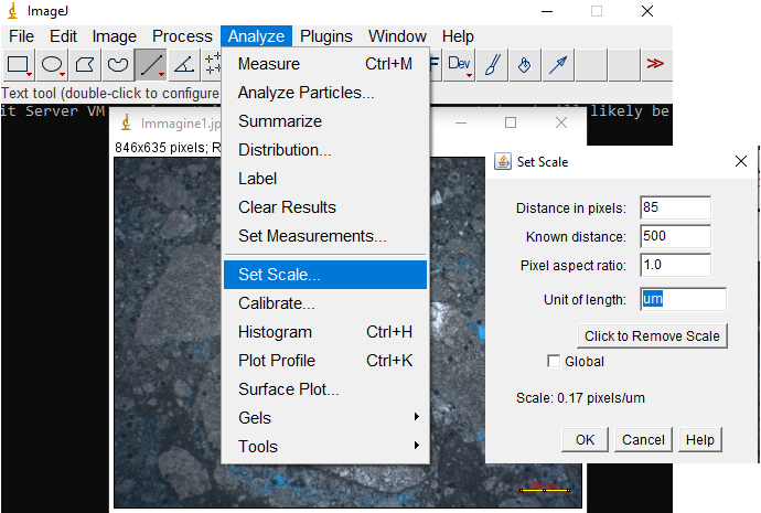
Figure 3.1: measurement scale setting operation
In this way the program associates the dimensions of the single pixel of the image with the relative micrometric dimensions adopted. It is then necessary to use the commands of the Image tool, first transforming the image into 8-bit to remove the colors and make everything in grayscale and then applying a threshold filter that allows the program to identify the individual within the image elements (clasts). Playing with the application bars, we make the clasts black and the background and voids white (Fig. 3.2).
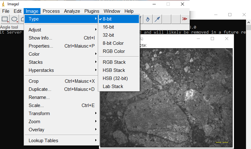
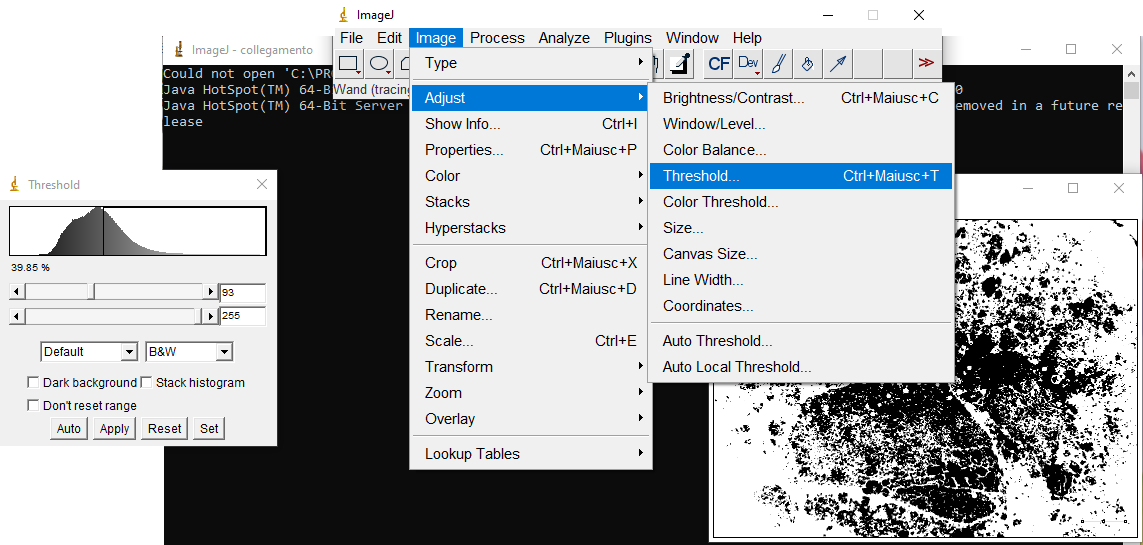
Figure 3.2: above, elimination of color scales; below application of the threshold filter
After having adjusted and redefined the edges of the elements and the cracks inside them with the drawing tools, we proceeded by processing the image making it binary, filtering out the noise and opening and closing the binary filters. The image will increasingly resemble the original photo (Fig.3.3).
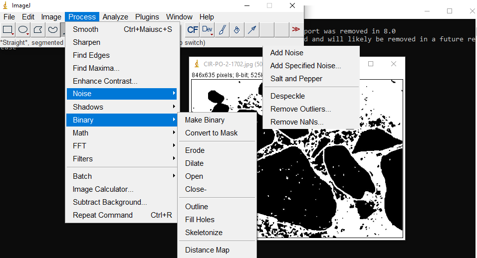
Figure 3.3: image processing
The image is ready for the geometric analysis, so from Analyze / set measures tool, we check all the measurement parameters that we want to obtain, both in view of the procedure necessary for the fractal analysis, and to obtain a restitution table of the parameters necessary for the calculation of the Ds parameter through Matlab. From the Analyze particles tool, setting the consideration of the edges in the bar, you start the procedure for identifying the calculation areas, which returns a .csv table and an image of the elements actually found by the program (Fig.3.4).
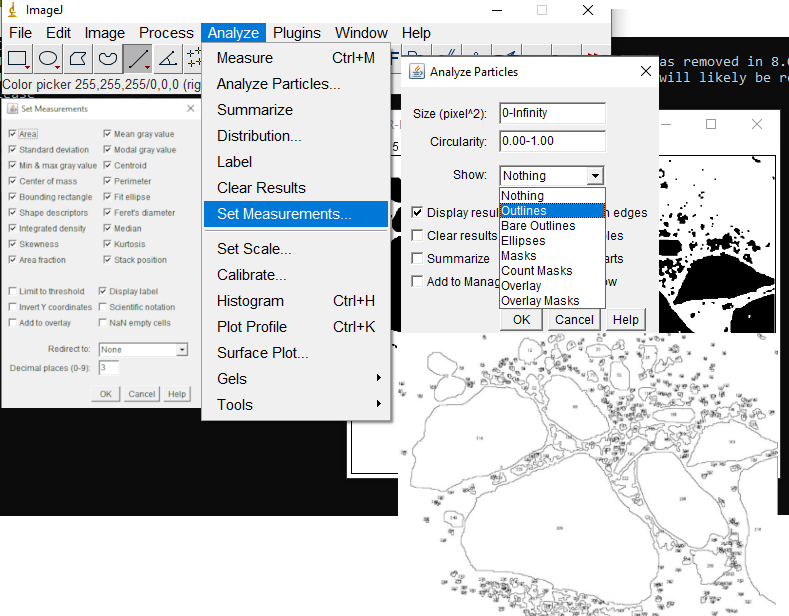
Figure 3.4: analysis settings setting and results
Through the Fractal box counter tool, you can start the fractal analysis procedure, based on the count of the number of times each clast crosses one of the edges of the square grid with an increasingly larger side processed by the software. The result of the analysis will be the plotting of a logarithmic graph that relates the square grid with the number of crossings. The angular coefficient of the regression line of the point analysis represents the parameter Dr (Fig.3.5).
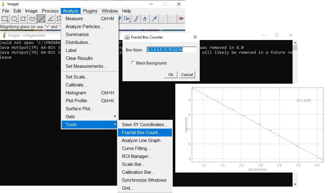
Figure 3.5: Fractal analysis and resulting plot
3.4.2 Matlab
MATLAB (abbreviation of Matrix Laboratory) is an environment for numerical computation and statistical analysis written in C, which also includes the homonymous programming language created by MathWorks and appears as a programming and numerical computation platform used for analysis data, algorithm development, and modeling by combining an optimized desktop environment for iterative analysis and design processes with a programming language that expresses mathematical operations with matrices and arrays directly. Matlab was used in this data processing phase to obtain the Ds parameter starting from the .csv table, suitably processed and transformed into a .txt text file easily readable by the program, obtained through image analysis with ImageJ. The code (CATAMORPH) gives us the plotting of a power low curve defined on the basis of the diameters and the cumulative frequency of the number of existing clasts with a diameter greater than the corresponding one on the abscissas. By working only on the central part of the curve to eliminate out-of-resolution values because they are too small or too large, a single trend line is identified, whose angular coefficient is precisely the parameter Ds.