Chapter 6 Implementation in R
Note: Before beginning any sensitivity analyses, please ensure that you have created an indicator variable for loss to follow-up (i.e., outcome missingness). In this worked example, the missingness indicator is named na_flag.
Basic descriptive statistics
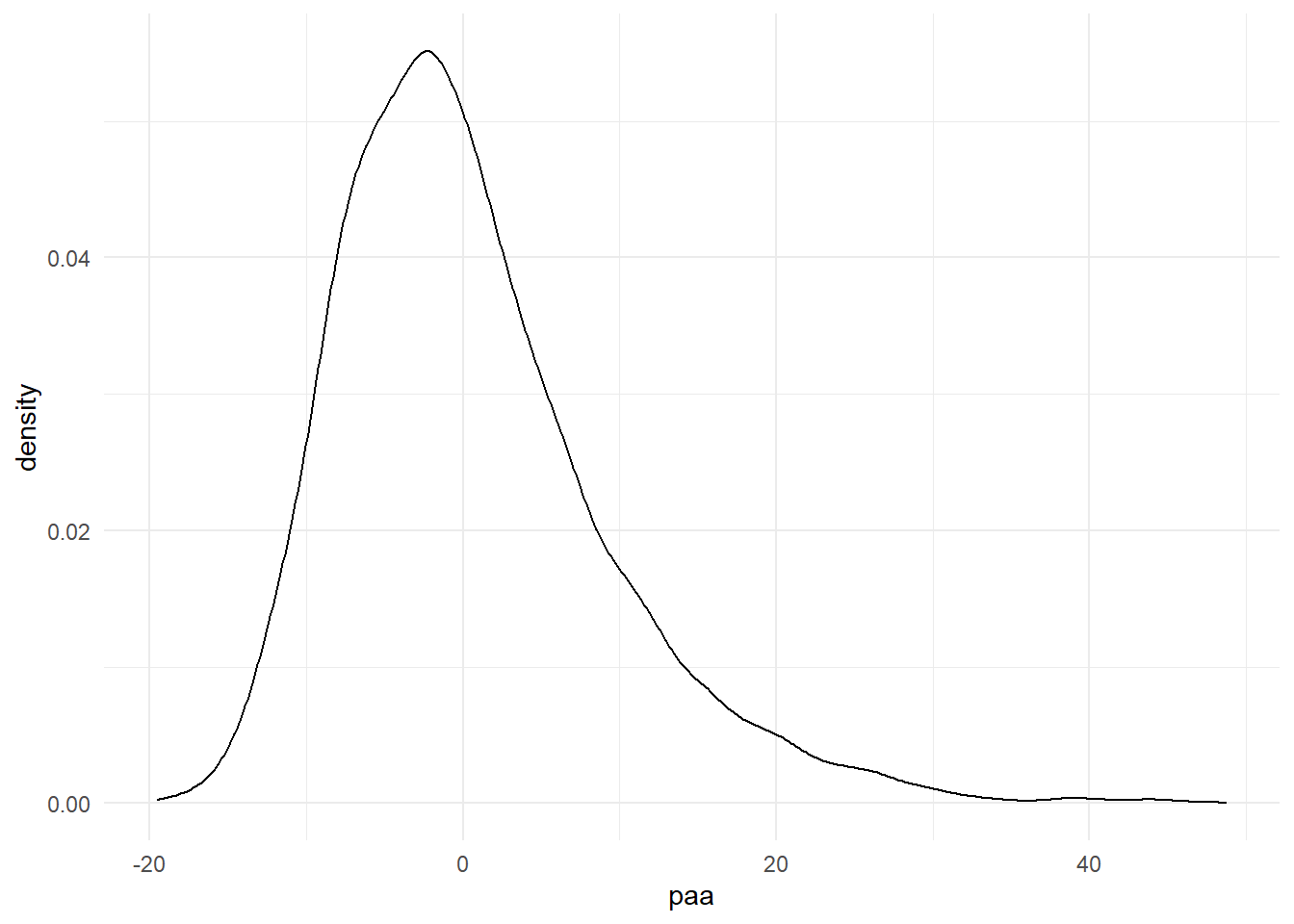
First, get to know your data by assess the degree of loss to follow-up and outcome distribution among complete cases in your dataset.
Number of observations in dataset:
nrow(HRS_df)= 9253Proportion of missing outcome data:
sum(is.na(HRS_df$paa))/nrow(HRS_df)= 0.1536799Outcome distribution in non-missing data:
HRS_df %>% ggplot() + geom_density(aes(x=paa)) + theme_minimal()
6.1 Scenario 1: Loss to follow-up unrelated to exposure, outcome, and confounders (MCAR)

DAG Scenario 1 (MCAR)
Approach: Under an MCAR assumption, we assume that study participants not lost to follow-up are a simple random sample of the original study population. As such, we can simply perform a complete case analysis of our data:
lm(paa ~ rawwealth + age + sex + raracem, data = HRS_df) %>%
  broom::tidy(conf.int = T) %>%
  filter(term == "rawwealth") %>%
knitr::kable(bootstrap_options = "condensed")| term | estimate | std.error | statistic | p.value | conf.low | conf.high |
|---|---|---|---|---|---|---|
| rawwealth | -0.0130595 | 0.0012304 | -10.61401 | 0 | -0.0154715 | -0.0106476 |
We find that \(RR=-0.0131\). In the context of our study, we interpret this to mean that a $10,000 increase in total wealth is associated with a 0.013 year decrease in biological-age advancement, adjusting for age, race, and sex (95%CI: -0.0155,-0.0106).
6.2 Scenario 2: Loss to follow-up differential by exposure \(A\) and/or measured confounder \(C\) (MAR)

DAG Scenario 2 (MAR)
Approach: Under an MAR missing data mechanism, we assume that study participants not lost to follow-up are exchangeable with those lost to follow-up, conditional on measured variables (exposure and/or covariates). Below, we use multiple imputation to impute our missing outcome values, using all available variables in our dataset (except our outcome missingness indicator). Other multiple imputation methods that account for the uncertainty of imputed values (e.g. joint multivariate normal imputation) may also be used.
MAR_step = mice(HRS_df, m=5, method = "norm.predict", quickpred(HRS_df, exc = "na_flag"), seed = 918, ridge = 0.0001)
# Note that variables can be included in/excluded from the imputation within the `quickpred` argument*
MAR_imputation =
with(MAR_step, lm(paa ~ rawwealth + age + sex + raracem))broom::tidy(pool(MAR_imputation), conf.int = T) %>%
select(term, estimate, std.error, statistic, p.value, conf.low, conf.high) %>%
filter(term == "rawwealth") %>%
knitr::kable(bootstrap_options = "condensed")| term | estimate | std.error | statistic | p.value | conf.low | conf.high |
|---|---|---|---|---|---|---|
| rawwealth | -0.0133753 | 0.0011294 | -11.84303 | 0 | -0.0155891 | -0.0111614 |
We find that \(RR=-0.0134\). We can interpret this to mean that assuming that outcome data are missing under an MAR mechanism and adjusting for age, race, and sex, a $10,000 increase in total wealth is associated with a 0.013 year decrease in biological-age advancement (95%CI: -0.0156,-0.0111).
6.3 Scenario 3: Loss to follow-up differential on disease/ disease + exposure status (MNAR)

DAG Scenario 3 (MNAR)
Approach: Under an MNAR missing data mechanism where loss to follow-up is conditional on the outcome, we assume that study participants lost to follow-up are not exchangeable with those not lost to follow-up; the true relationship between exposure and outcome differs between the two groups based on the (unmeasured) outcome variable. To model this missing data mechanism, we extend the MAR scenario by modifying all imputed observations by a constant additive or multiplicative constant (\(\delta\) or \(c\)). Below, we show the implementation of each method in the following steps:
- We provide a simple example testing a single additive \(\delta\) or multiplicative parameter \(c\) by which we think missing and non-missing outcomes differ
- We demonstrate how to iterate this process over a range of \(\delta\) or \(c\) parameters to test the sensitivity of our results to different MNAR assumptions
- We provide sample output to be used in reporting sensitivity analyses.
Scenario 3a: Additive relationship between Y and data missingness (\(\delta\) method)
Use case
In this scenario, we assume that people who are lost to follow-up have 3 additional years of biological-age advancement compared to people who are not lost to follow-up
We integrate this “prior” into our model by adding 3 years of biological-age advancement to all imputed values in our dataset (using an
ifelsestatement conditional on our missingness indicator variablena_flag)Finally, we proceed to estimate our pooled effect-size parameter of interest (in this case, the risk ratio) in the same way we generated our previous multiply imputed dataset under an MAR assumption
MNAR_conversion_3a =
  complete(MAR_step, action='long', include=TRUE) %>%
  mutate(paa = ifelse(na_flag == 1, paa+3, paa))

MNAR_data_3a = as.mids(MNAR_conversion_3a)

MNAR_output_3a =
  with(MNAR_data_3a, lm(paa ~ rawwealth + age + sex + raracem))

params_3a =
  broom::tidy(pool(MNAR_output_3a), conf.int = T) %>%
  select(term, estimate, std.error, statistic, p.value, conf.low, conf.high) %>%
  filter(term == "rawwealth")

desc_3a = with(MNAR_data_3a, expr=c("Y_mean"=mean(paa), "Y_sd"=stats::sd(paa)))
desc_3a = withPool_MI(desc_3a) %>% as.data.frame() %>% t()

rownames(desc_3a) <- c()

cbind(params_3a, desc_3a) %>%
knitr::kable(bootstrap_options = "condensed") | term | estimate | std.error | statistic | p.value | conf.low | conf.high | Y_mean | Y_sd |
|---|---|---|---|---|---|---|---|---|
| rawwealth | -0.0133208 | 0.0011389 | -11.69658 | 0 | -0.0155533 | -0.0110884 | 0.9307468 | 8.633165 |
We find that \(RR=-0.0133\). Assuming that people who are lost to follow-up have 3 additional years of biological-age advancement compared to people who are not lost to follow-up, and adjusting for age, race, and sex, a $10,000 increase in total wealth is associated with a 0.013 year decrease in biological-age advancement (95%CI: -0.0156,-0.0111).
Iterating over a range of values
Having demonstrated the logic underlying a single case, we now proceed to iterate our sensitivity analysis over a range of \(\delta\) values. See Section 5 for a discussion on how to select a range of values to test.
To iterate over a range of \(\delta\) values, we proceed as follows (each step is labelled in the code below):
We write a function with the delta parameter as the function input.
We create a vector specifying a range of plausible delta values
We run this vector of plausible delta values through the function written in Step 1.
# Write function to obtain estimate under given delta parameter
delta_MNAR_f = function(delta){

  MAR_step = mice(HRS_df, m=5, method = "pmm", quickpred(HRS_df, exc = "na_flag"), seed = 918)

  MNAR_conversion_delta =
    complete(MAR_step, action='long', include=TRUE) %>%
    mutate(paa = ifelse(na_flag == 1, paa + delta, paa))

  MNAR_data_delta = as.mids(MNAR_conversion_delta)

  output_delta =
    with(MNAR_data_delta, lm(paa ~ rawwealth + age + sex + raracem))

  params_delta =
    summary(pool(output_delta)) %>%
    filter(term == "rawwealth")

  desc_delta = with(MNAR_data_delta, expr=c("Y_mean"=mean(paa), "Y_sd"=stats::sd(paa)))
  desc_delta = withPool_MI(desc_delta) %>% as.data.frame() %>% t()

  cbind(params_delta, desc_delta)

}

# Set range of plausible delta values
delta_inputs = c(-32, -16, -8, -4, -2, -1, 0, 1, 2, 4, 8, 16, 32, 64)

# Map output
output_delta =
  map_df(delta_inputs, delta_MNAR_f)

rownames(output_delta) <- c()
Output
We can show our output in tabular and graphical form, as follows. In the output table, note that we have added two additional columns showing the mean and standard deviation of each outcome under each MNAR condition:
output_formatted_delta =
  cbind(delta_inputs, output_delta) %>%
  select(-term) %>%
  mutate(across(c("estimate":"std.error"), round, 3),
         across(c("statistic":"df", "Y_mean":"Y_sd"), round, 2),
         p.value = scientific(p.value, digits = 2))

output_formatted_delta %>%
knitr::kable(bootstrap_options = "condensed")| delta_inputs | estimate | std.error | statistic | df | p.value | Y_mean | Y_sd |
|---|---|---|---|---|---|---|---|
| -32 | -0.014 | 0.002 | -7.18 | 9022.21 | 7.5e-13 | -4.45 | 14.41 |
| -16 | -0.014 | 0.001 | -9.86 | 8483.75 | 0.0e+00 | -1.99 | 10.37 |
| -8 | -0.014 | 0.001 | -11.21 | 8014.03 | 0.0e+00 | -0.76 | 9.08 |
| -4 | -0.013 | 0.001 | -11.62 | 7830.24 | 0.0e+00 | -0.14 | 8.73 |
| -2 | -0.013 | 0.001 | -11.72 | 7778.00 | 0.0e+00 | 0.16 | 8.64 |
| -1 | -0.013 | 0.001 | -11.73 | 7764.44 | 0.0e+00 | 0.32 | 8.62 |
| 0 | -0.013 | 0.001 | -11.73 | 7759.80 | 0.0e+00 | 0.47 | 8.61 |
| 1 | -0.013 | 0.001 | -11.70 | 7764.18 | 0.0e+00 | 0.62 | 8.62 |
| 2 | -0.013 | 0.001 | -11.66 | 7777.48 | 0.0e+00 | 0.78 | 8.64 |
| 4 | -0.013 | 0.001 | -11.50 | 7829.25 | 0.0e+00 | 1.08 | 8.73 |
| 8 | -0.013 | 0.001 | -10.97 | 8012.40 | 0.0e+00 | 1.70 | 9.08 |
| 16 | -0.013 | 0.001 | -9.45 | 8482.15 | 0.0e+00 | 2.93 | 10.36 |
| 32 | -0.013 | 0.002 | -6.59 | 9021.72 | 4.7e-11 | 5.39 | 14.39 |
| 64 | -0.012 | 0.003 | -3.65 | 9212.80 | 2.6e-04 | 10.31 | 24.63 |
In graphical form, we show how our \(RR\) point estimate changes at each value of \(\delta\). The null value of 0 is indicated with a red dotted line.
output_delta %>%
  ggplot(aes(x = delta_inputs, y = estimate)) +
  geom_smooth() +
  geom_point() +
  geom_hline(yintercept=0, linetype="dashed", color = "red") +
  theme_minimal()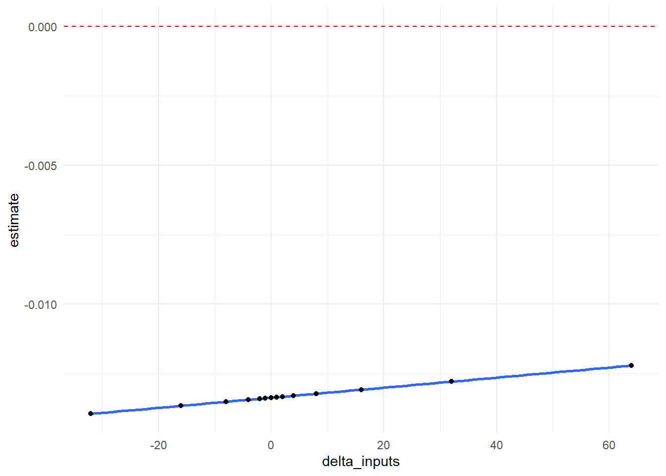
Scenario 3b: Multiplicative relationship between Y and data missingness (\(c\) scale method)
Use case
In this scenario, we assume that people who are lost to follow-up have 1.5 times the biological-age advancement compared to people who are not lost to follow-up
We integrate this “prior” into our model by multiplying all imputed values of biological-age advancement in our dataset by 1.5 (using an
ifelsestatement conditional on our missingness indicator variablena_flag)Finally, we proceed to estimate our pooled effect-size parameter of interest (in this case, the risk ratio) in the same way we generated our previous multiply imputed dataset under an MAR assumption
MNAR_conversion_3b =
  complete(MAR_step, action='long', include=TRUE) %>%
  mutate(paa = ifelse(na_flag == 1, paa*1.5, paa))

MNAR_data_3b = as.mids(MNAR_conversion_3b)

MNAR_output_3b =
  with(MNAR_data_3b, lm(paa ~ rawwealth + age + sex + raracem))

params_3b =
  broom::tidy(pool(MNAR_output_3b), conf.int = T) %>%
  select(term, estimate, std.error, statistic, p.value, conf.low, conf.high) %>%
  filter(term == "rawwealth")

desc_3b = with(MNAR_data_3b, expr=c("Y_mean"=mean(paa), "Y_sd"=stats::sd(paa)))
desc_3b = withPool_MI(desc_3b) %>% as.data.frame() %>% t()

rownames(desc_3b) <- c()

cbind(params_3b, desc_3b) %>%
knitr::kable(bootstrap_options = "condensed") | term | estimate | std.error | statistic | p.value | conf.low | conf.high | Y_mean | Y_sd |
|---|---|---|---|---|---|---|---|---|
| rawwealth | -0.014446 | 0.0012203 | -11.83781 | 0 | -0.0168381 | -0.0120539 | 0.5037383 | 9.262329 |
We find that \(RR=-0.0145\). Assuming that people who are lost to follow-up have 1.5 times the biological-age advancement of to people who are not lost to follow-up, and adjusting for age, race, and sex, a $10,000 increase in total wealth is associated with a 0.015 year decrease in biological-age advancement (95%CI: -0.0169,-0.0120).
Iterating over a range of values
Having demonstrated the logic underlying a single case, we now proceed to iterate our sensitivity analysis over a range of \(c\) values. See Section 5 for a discussion on how to select a range of values to test.
To iterate over a range of \(c\) values, we proceed as follows (each step is labelled in the code below):
We write a function with the scale parameter \(c\) as the function input.
We create a vector specifying a range of plausible scale values \(c\)
We run this vector of plausible scale values through the function written in Step 1.
# Write function to obtain estimate under given scale parameter
scale_MNAR_f = function(scale){

  MAR_step = mice(HRS_df, m=5, method = "pmm", quickpred(HRS_df, exc = "na_flag"), seed = 918)

  MNAR_conversion_scale =
    complete(MAR_step, action='long', include=TRUE) %>%
    mutate(paa = ifelse(na_flag == 1, paa + scale, paa))

  MNAR_data_scale = as.mids(MNAR_conversion_scale)

  output_scale =
    with(MNAR_data_scale, lm(paa ~ rawwealth + age + sex + raracem))

  params_scale =
    summary(pool(output_scale)) %>%
    filter(term == "rawwealth")

  desc_scale = with(MNAR_data_scale, expr=c("Y_mean"=mean(paa), "Y_sd"=stats::sd(paa)))
  desc_scale = withPool_MI(desc_scale) %>% as.data.frame() %>% t()

  cbind(params_scale, desc_scale)

}

# Set range of plausible scale values
scale_inputs = c(-32, -16, -8, -4, -2, -1, 0, 1, 2, 4, 8, 16, 32)

# Map output
output_scale =
  map_df(scale_inputs, scale_MNAR_f)

rownames(output_scale) <- c()
Output
We can show our output in tabular and graphical form, as follows. In the output table, note that we have added two additional columns showing the mean and standard deviation of each outcome under each MNAR condition:
output_formatted_scale =
  cbind(scale_inputs, output_scale) %>%
  select(-term) %>%
  mutate(across(c("estimate":"std.error"), round, 3),
         across(c("statistic":"df", "Y_mean":"Y_sd"), round, 2),
         p.value = scientific(p.value, digits = 2))

output_formatted_scale %>%
knitr::kable(bootstrap_options = "condensed")| scale_inputs | estimate | std.error | statistic | df | p.value | Y_mean | Y_sd |
|---|---|---|---|---|---|---|---|
| -32 | -0.014 | 0.002 | -7.18 | 9022.21 | 7.5e-13 | -4.45 | 14.41 |
| -16 | -0.014 | 0.001 | -9.86 | 8483.75 | 0.0e+00 | -1.99 | 10.37 |
| -8 | -0.014 | 0.001 | -11.21 | 8014.03 | 0.0e+00 | -0.76 | 9.08 |
| -4 | -0.013 | 0.001 | -11.62 | 7830.24 | 0.0e+00 | -0.14 | 8.73 |
| -2 | -0.013 | 0.001 | -11.72 | 7778.00 | 0.0e+00 | 0.16 | 8.64 |
| -1 | -0.013 | 0.001 | -11.73 | 7764.44 | 0.0e+00 | 0.32 | 8.62 |
| 0 | -0.013 | 0.001 | -11.73 | 7759.80 | 0.0e+00 | 0.47 | 8.61 |
| 1 | -0.013 | 0.001 | -11.70 | 7764.18 | 0.0e+00 | 0.62 | 8.62 |
| 2 | -0.013 | 0.001 | -11.66 | 7777.48 | 0.0e+00 | 0.78 | 8.64 |
| 4 | -0.013 | 0.001 | -11.50 | 7829.25 | 0.0e+00 | 1.08 | 8.73 |
| 8 | -0.013 | 0.001 | -10.97 | 8012.40 | 0.0e+00 | 1.70 | 9.08 |
| 16 | -0.013 | 0.001 | -9.45 | 8482.15 | 0.0e+00 | 2.93 | 10.36 |
| 32 | -0.013 | 0.002 | -6.59 | 9021.72 | 4.7e-11 | 5.39 | 14.39 |
In graphical form, we show how our \(RR\) point estimate changes at each value of \(\delta\). The null value of 0 is indicated with a red dotted line.
output_scale %>%
  ggplot(aes(x = scale_inputs, y = estimate)) +
  geom_smooth() +
  geom_point() +
  geom_hline(yintercept=0, linetype="dashed", color = "red") +
  theme_minimal()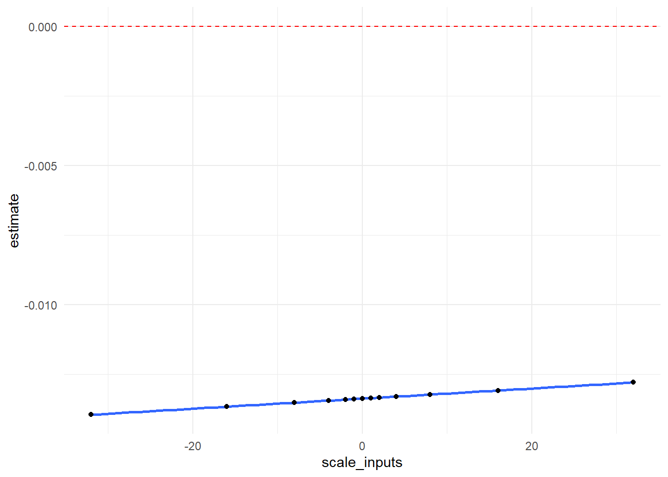
6.4 Scenario 4: Loss to follow-up differential on unmeasured confounder (MNAR)

DAG Scenario 4 (MNAR)
Under an MNAR missing data mechanism where we loss to follow-up is conditional on the outcome, we assume that study participants lost to follow-up are not exchangeable with those not lost to follow-up; the true relationship between exposure and outcome differs between the two groups based on an unmeasured common cause of exposure and disease.
In thie case, there are the following relationships to specify:
The confounder-exposure relationship
The confounder-disease relationship
The confounder-missingness relationship
Below, we show the implementation of sensitivity analyses for an unmeasured confounder causing Y as follows:
We generate several unmeasured confounders using the MAR-imputed dataset (this serves to vary the \(A-U\) and \(Y-U\) relationship)
We create a vector of offset terms to define the relationship between U and missingness (this serves to vary the \(U-LTFU\) relationship)
We provide example code to iterate over these unmeasured confounders to demonstrate their effect on the causal effect estimate given a range of associations between each confounder and outcome missingness
Example and sample code
Generating unmeasured confounders:
We generate an unmeasured confounder \(U\), expressed as a function of both exposure \(A\) and disease \(Y\) (Generating the confounder variable as a function of exposure and disease might seem strange, as it would seem that we are creating a collider variable. However, because we are hypothesizing in our sensitivity analyses that the observed \(A-Y\) relationship is not the “true” causal effect, we can generate U without concerning ourselves with directionality; the magnitude of the \(A-U\) and \(Y-U\) relationships are our primary concern.)
Below, we create several potential unmeasured confounders (\(U1\), \(U2\), \(U3\)) as a function of exposure and disease in our MAR-imputed dataset. You may create as many \(U\) variables as desired.
MAR_step = mice(HRS_df, m=5, method = "pmm", quickpred(HRS_df, exc = "na_flag"), seed = 918)

imputed_long_df =
  complete(MAR_step, action='long', include=TRUE) %>%
  mutate(U1 = (((rawwealth+15000)/5000) + (1.5*paa)),
         U2 = (((rawwealth+15000)/5000) + (2.5*paa)),
         U3 = (((rawwealth+15000)/5000) + (3.5*paa))
         )
After having generated the variable, we generate descriptive statistics for \(U\) and test \(U\)-exposure and \(U\)-disease relationships:
imputed_MAR_df =
  as.mids(imputed_long_df)

# Calculate mean of outcome and unmeasured confounders using imputed data
desc_U = with(imputed_MAR_df, expr=c("Y_mean"=mean(paa), "Y_sd"=sd(paa),
                                      "U1_mean"=mean(U1), "U1_sd"=sd(U1),
                                      "U2_mean"=mean(U2), "U2_sd"=sd(U2),
                                      "U3_mean"=mean(U3), "U3_sd"=sd(U3)))

desc_U = withPool_MI(desc_U) %>% as.data.frame()
desc_U %>%
knitr::kable(caption = "Mean and standard deviation of outcome and unmeasured confounders")| . | |
|---|---|
| Y_mean | 0.4700495 |
| Y_sd | 8.6107036 |
| U1_mean | 3.7127219 |
| U1_sd | 12.9141038 |
| U2_mean | 4.1827714 |
| U2_sd | 21.5248036 |
| U3_mean | 4.6528209 |
| U3_sd | 30.1355056 |
# Calculate exposure-confounder associations for all U variables
EC_model_U1 =
    with(imputed_MAR_df, lm(rawwealth ~ U1))
EC_model_U1 =
  summary(pool(EC_model_U1)) %>%
  filter(term == "U1")

EC_model_U2 =
    with(imputed_MAR_df, lm(rawwealth ~ U2))
EC_model_U2 =
  summary(pool(EC_model_U2)) %>%
  filter(term == "U2")

EC_model_U3 =
    with(imputed_MAR_df, lm(rawwealth ~ U3))
EC_model_U3 =
  summary(pool(EC_model_U3)) %>%
  filter(term == "U3")

EC_models_summary =
  rbind(EC_model_U1, EC_model_U2)
EC_models_summary =
  rbind(EC_models_summary, EC_model_U3)

EC_models_summary %>%
  select(term, estimate, std.error) %>%
  rename(variable = term,
         RR = estimate) %>%
knitr::kable(bootstrap_options = "condensed", caption = "Risk Ratios, U-A relationship")| variable | RR | std.error |
|---|---|---|
| U1 | -0.7520250 | 0.0625914 |
| U2 | -0.4529040 | 0.0375505 |
| U3 | -0.3240197 | 0.0268205 |
# Calculate disease-confounder associations for all U variables
DC_model_U1 =
    with(imputed_MAR_df, lm(paa ~ U1))
DC_model_U1 =
  summary(pool(DC_model_U1)) %>%
  filter(term == "U1")

DC_model_U2 =
    with(imputed_MAR_df, lm(paa ~ U2))
DC_model_U2 =
  summary(pool(DC_model_U2)) %>%
  filter(term == "U2")

DC_model_U3 =
    with(imputed_MAR_df, lm(paa ~ U3))
DC_model_U3 =
  summary(pool(DC_model_U3)) %>%
  filter(term == "U3")

DC_models_summary =
  rbind(DC_model_U1, DC_model_U2)
DC_models_summary =
  rbind(DC_models_summary, DC_model_U3)

DC_models_summary %>%
  select(term, estimate, std.error) %>%
  rename(variable = term,
         RR = estimate) %>%
knitr::kable(bootstrap_options = "condensed", caption = "Risk Ratios, U-Y relationship")| variable | RR | std.error |
|---|---|---|
| U1 | 0.6667669 | 8.3e-06 |
| U2 | 0.4000362 | 3.0e-06 |
| U3 | 0.2857328 | 1.5e-06 |
Defining the confounder-missingness relationship
As in scenario 6.3, we then modify imputed outcome values by an offset parameter (which is represented as a function of our unmeasured confounder):
# Write function to obtain estimate under given scale parameter
MNAR_U_f = function(scale, u_var){

  imputed_long_df =
    imputed_long_df %>%
    mutate(paa = ifelse(na_flag == 1, paa + scale*pull(imputed_long_df, u_var), paa))

  MNAR_data_scale = as.mids(imputed_long_df)

  output_scale =
    with(MNAR_data_scale, lm(paa ~ rawwealth + age + sex + raracem))

  params_scale =
    summary(pool(output_scale)) %>%
    filter(term == "rawwealth")

  desc_scale = with(MNAR_data_scale, expr=c("Y_mean"=mean(paa), "Y_sd"=stats::sd(paa)))
  desc_scale = withPool_MI(desc_scale) %>% as.data.frame() %>% t()

  cbind(params_scale, desc_scale)

}

# Set range of plausible scale values
scale_inputs = c(-3.2, -1.6, -.8, -.4, -.2, -.1, 0, .1, .2, .4, .8, 1.6, 3.2)

# Create vector of all U variables
u_inputs = c("U1", "U2", "U3")

# Create cross of those two vectors for model inputs
MNAR_U_inputs = crossing(u_inputs, scale_inputs)

# Map and format output
output_U =
  map2_df(MNAR_U_inputs$scale_inputs, MNAR_U_inputs$u_inputs, MNAR_U_f)

output_U =
  cbind(MNAR_U_inputs, output_U)
Output
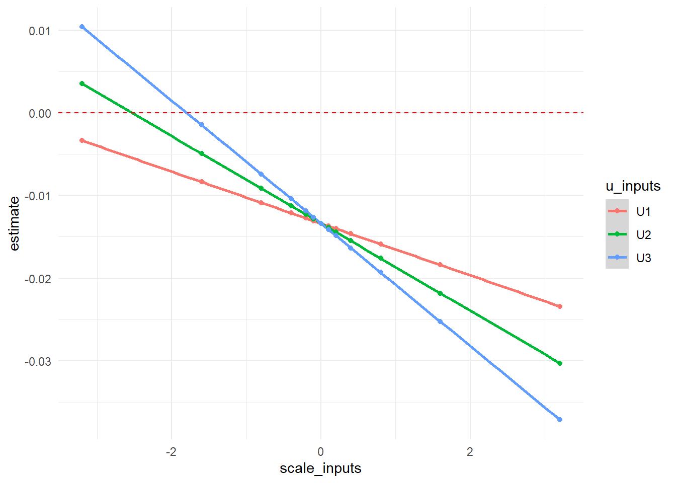
We can show our output in tabular and graphical form, as follows. Note that we have added two additional columns showing the mean and standard deviation of each outcome under each MNAR condition:
output_U_formatted =
  output_U %>%
  select(-term) %>%
  mutate(across(c("estimate":"std.error"), round, 3),
         across(c("statistic":"df", "Y_mean", "Y_sd"), round, 2),
         p.value = scientific(p.value, digits = 2))

rownames(output_U_formatted) <- c()

output_U_formatted %>%
knitr::kable(bootstrap_options = "condensed")| u_inputs | scale_inputs | estimate | std.error | statistic | df | p.value | Y_mean | Y_sd |
|---|---|---|---|---|---|---|---|---|
| U1 | -3.2 | -0.003 | 0.002 | -1.57 | 2225.66 | 1.2e-01 | -1.34 | 15.35 |
| U1 | -1.6 | -0.008 | 0.001 | -6.51 | 6370.78 | 7.9e-11 | -0.43 | 9.43 |
| U1 | -0.8 | -0.011 | 0.001 | -10.11 | 9237.88 | 0.0e+00 | 0.02 | 8.06 |
| U1 | -0.4 | -0.012 | 0.001 | -11.31 | 9175.19 | 0.0e+00 | 0.24 | 8.09 |
| U1 | -0.2 | -0.013 | 0.001 | -11.62 | 8756.31 | 0.0e+00 | 0.36 | 8.29 |
| U1 | -0.1 | -0.013 | 0.001 | -11.70 | 8326.93 | 0.0e+00 | 0.41 | 8.44 |
| U1 | 0.0 | -0.013 | 0.001 | -11.73 | 7759.80 | 0.0e+00 | 0.47 | 8.61 |
| U1 | 0.1 | -0.014 | 0.001 | -11.72 | 7102.98 | 0.0e+00 | 0.53 | 8.81 |
| U1 | 0.2 | -0.014 | 0.001 | -11.68 | 6416.81 | 0.0e+00 | 0.58 | 9.03 |
| U1 | 0.4 | -0.015 | 0.001 | -11.52 | 5146.95 | 0.0e+00 | 0.70 | 9.54 |
| U1 | 0.8 | -0.016 | 0.001 | -11.00 | 3435.11 | 0.0e+00 | 0.92 | 10.78 |
| U1 | 1.6 | -0.018 | 0.002 | -9.82 | 2104.01 | 0.0e+00 | 1.37 | 13.83 |
| U1 | 3.2 | -0.023 | 0.003 | -8.14 | 1500.01 | 8.9e-16 | 2.28 | 20.99 |
| U2 | -3.2 | 0.004 | 0.003 | 1.02 | 1465.29 | 3.1e-01 | -1.56 | 24.68 |
| U2 | -1.6 | -0.005 | 0.002 | -2.77 | 2622.85 | 5.7e-03 | -0.54 | 12.86 |
| U2 | -0.8 | -0.009 | 0.001 | -7.79 | 7898.30 | 7.5e-15 | -0.04 | 8.69 |
| U2 | -0.4 | -0.011 | 0.001 | -10.61 | 9243.86 | 0.0e+00 | 0.22 | 7.99 |
| U2 | -0.2 | -0.012 | 0.001 | -11.44 | 9092.04 | 0.0e+00 | 0.34 | 8.14 |
| U2 | -0.1 | -0.013 | 0.001 | -11.65 | 8629.81 | 0.0e+00 | 0.41 | 8.34 |
| U2 | 0.0 | -0.013 | 0.001 | -11.73 | 7759.80 | 0.0e+00 | 0.47 | 8.61 |
| U2 | 0.1 | -0.014 | 0.001 | -11.71 | 6643.99 | 0.0e+00 | 0.53 | 8.95 |
| U2 | 0.2 | -0.014 | 0.001 | -11.60 | 5538.38 | 0.0e+00 | 0.60 | 9.36 |
| U2 | 0.4 | -0.015 | 0.001 | -11.23 | 3867.76 | 0.0e+00 | 0.72 | 10.32 |
| U2 | 0.8 | -0.018 | 0.002 | -10.28 | 2341.25 | 0.0e+00 | 0.98 | 12.69 |
| U2 | 1.6 | -0.022 | 0.003 | -8.72 | 1551.69 | 0.0e+00 | 1.48 | 18.33 |
| U2 | 3.2 | -0.030 | 0.004 | -7.12 | 1274.12 | 1.8e-12 | 2.50 | 30.83 |
| U3 | -3.2 | 0.010 | 0.005 | 2.15 | 1296.35 | 3.2e-02 | -1.78 | 34.67 |
| U3 | -1.6 | -0.001 | 0.002 | -0.62 | 1770.58 | 5.3e-01 | -0.65 | 17.22 |
| U3 | -0.8 | -0.007 | 0.001 | -5.44 | 4750.70 | 5.7e-08 | -0.09 | 9.99 |
| U3 | -0.4 | -0.010 | 0.001 | -9.61 | 9177.70 | 0.0e+00 | 0.19 | 8.10 |
| U3 | -0.2 | -0.012 | 0.001 | -11.17 | 9218.57 | 0.0e+00 | 0.33 | 8.03 |
| U3 | -0.1 | -0.013 | 0.001 | -11.58 | 8864.18 | 0.0e+00 | 0.40 | 8.25 |
| U3 | 0.0 | -0.013 | 0.001 | -11.73 | 7759.80 | 0.0e+00 | 0.47 | 8.61 |
| U3 | 0.1 | -0.014 | 0.001 | -11.68 | 6187.66 | 0.0e+00 | 0.54 | 9.11 |
| U3 | 0.2 | -0.015 | 0.001 | -11.48 | 4768.74 | 0.0e+00 | 0.61 | 9.72 |
| U3 | 0.4 | -0.016 | 0.002 | -10.88 | 3040.69 | 0.0e+00 | 0.75 | 11.20 |
| U3 | 0.8 | -0.019 | 0.002 | -9.61 | 1854.99 | 0.0e+00 | 1.03 | 14.81 |
| U3 | 1.6 | -0.025 | 0.003 | -7.95 | 1359.10 | 4.0e-15 | 1.59 | 23.14 |
| U3 | 3.2 | -0.037 | 0.006 | -6.55 | 1203.58 | 8.3e-11 | 2.72 | 40.99 |
In graphical form, we show how our \(RR\) point estimate changes at each value of \(\delta\) with each potential unmeasured confounder as a different line. The null value of 0 is indicated with a red dotted line.
output_U %>%
  ggplot(aes(x = scale_inputs, y = estimate, color = u_inputs)) +
  geom_smooth() +
  geom_point() +
  geom_hline(yintercept=0, linetype="dashed", color = "red") +
  theme_minimal()