Chapter 10 Upcoming topics

10.1 FAQs

10.1.0.1 Testing for Normality

Testing for Normality of a variable can be described as testing to see if the data follows the Normal distribution. The most commonly used way to assess this is by visual inspection, either by plotting a Histogram (from the data) or by plotting a Q-Q plot (or Quantile-Quantile plot). The formal methods commonly used are the Shapiro-Wilk test and the Kolmogorov-Smirnov test.

10.1.0.1.1 Visual methods

When the data is plotted as a histogram, Normality is assessed by inspecting the shape of the histogram. Typically, if the histogram exhibits a bell-shape, the data is assumed to be Normal. The shape of the histogram can also indicate whether the distribution is skewed. For the Q-Q plot, Normality is assumed if the points on the plot follow (approximately) the diagonal line. In this case, the Q-Q plot is a scatterplot of the quantiles from the data plotted against theoretical, Normally distributed quantiles.

Try the following code to test the Haggis data for Normality.

library(ggplot2)
ba <- data.frame(c(before,after))
ba$timeframe <- c(rep("before",length(before)),rep("after",length(after)))
colnames(ba)<-c("number","timeframe")


# Histogram


ggplot(ba, aes(x = number)) + facet_wrap(. ~timeframe,ncol=1)+
  geom_histogram(binwidth=1,aes(fill = ..count..)) +
  scale_x_continuous(name = "Percentage of limpers per household")  +
  scale_y_continuous(name = "Count") +
  ggtitle("Percentage of limpers per Haggis household",
          subtitle="before and after physiotherapy")+
  theme(text = element_text(size=40))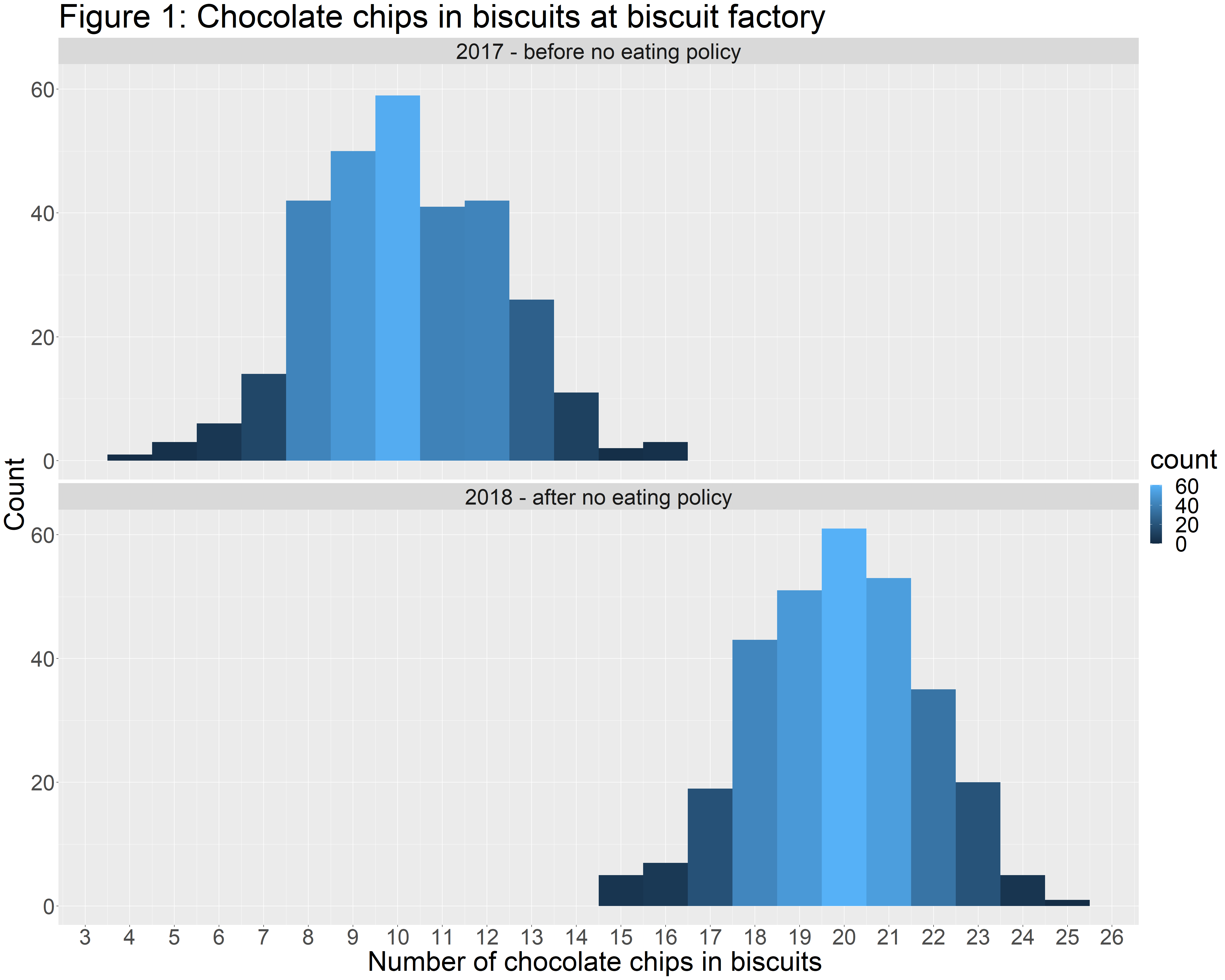

# Q-Q plot

qqnorm(before)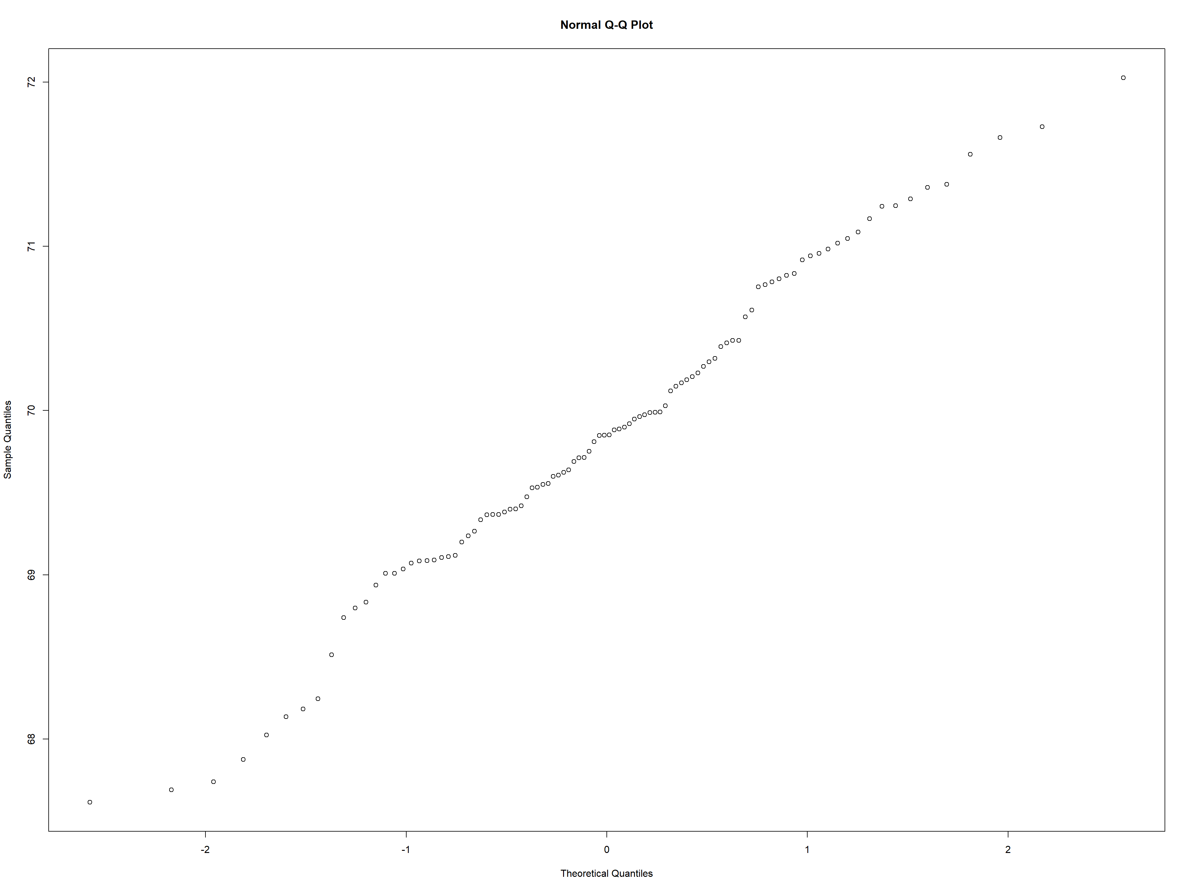

qqnorm(after)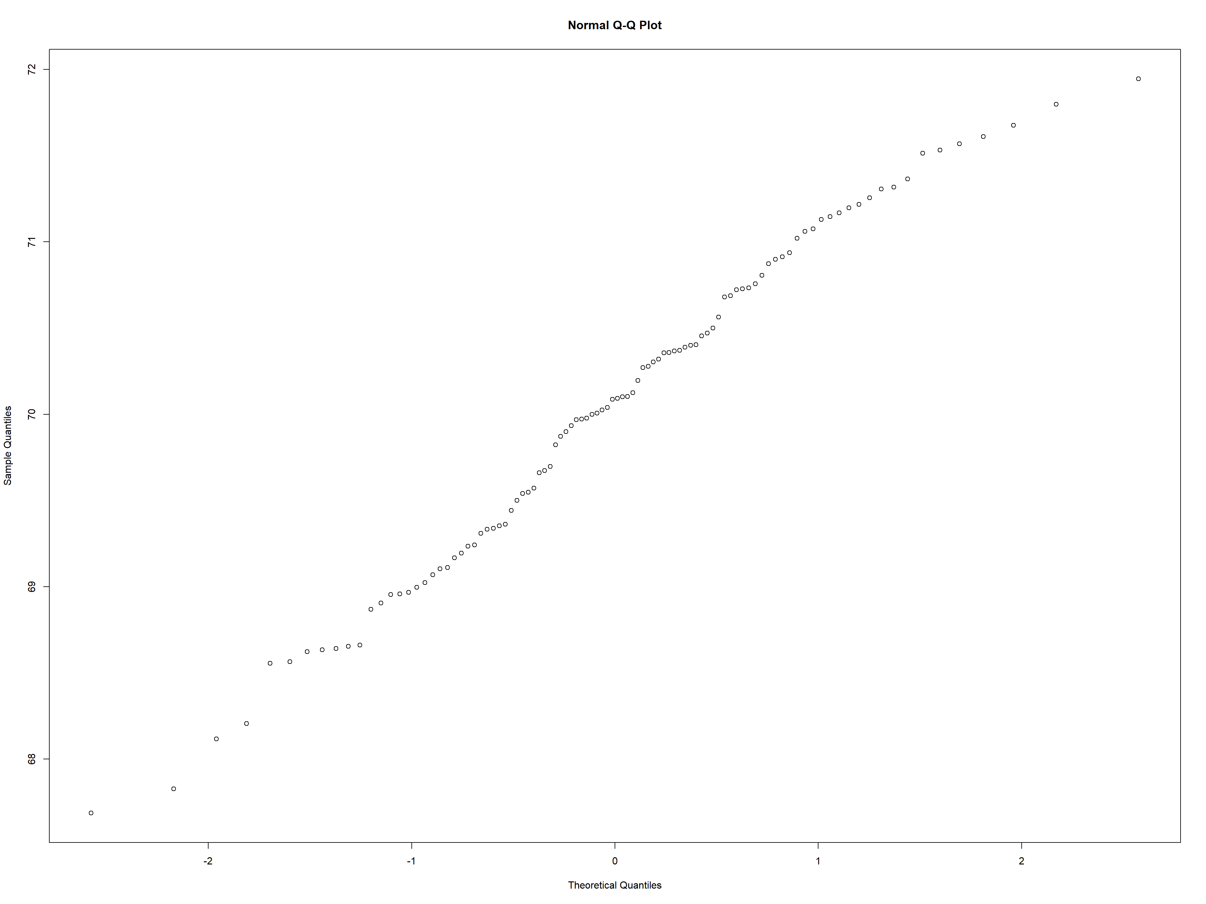

10.1.0.1.2 Formal methods

For both of the abovementioned formal methods, a p-value greater than 0.05 indicates that the data is Normally distributed.

Try the following code to test the Haggis data for Normality.

# Shapiro-Wilk test

shapiro.test(before)

## 
##  Shapiro-Wilk normality test
## 
## data:  before
## W = 0.99444, p-value = 0.958

# Kolgomorov test

ks.test(after, 'pnorm')

## 
##  One-sample Kolmogorov-Smirnov test
## 
## data:  after
## D = 1, p-value < 2.2e-16
## alternative hypothesis: two-sided