Chapter 6 Sensitivity Analysis 2

6.1 Data

rm(list=ls())
library(tidyverse)
library(purrr)
library(Metrics)
library(stringr)
library(MatrixModels)
library(sf)

load("./_dat/NL_VEN_dat_north.RData")

6.2 Municipios with no mining [in the North]

pop <- read.csv("./_dat/data_mal.csv") %>%
  filter(ESTADO == "Sucre") %>%
  dplyr::select(4:9,11,13,15) %>%
  gather(t, pob, pob_2014:c2017) %>%
  mutate(year = as.numeric(str_sub(t,-4,-1)),
         t = str_sub(t,1,1),
         CODIGO_INE = as.character(CODIGO_INE)) %>%
  spread(t,pob) %>%
  dplyr::rename(cases = c, pob = p)

vzla.sf <- st_read("./_dat/vzla_mun_mal2014_2/vzla_mun_mal2014_2.shp") %>%
  mutate(state = str_sub(CODIGO_INE,1,2)) %>%
  filter(state ==19)

vzla <- vzla.sf %>% 
  st_set_geometry(NULL) %>%
  dplyr:: rename(X2014 = Malaria__3,
                 X2015 = Malaria__5,
                 X2016 = Malaria__7,
                 X2017 = Malaria__9) %>%
  gather(year, cases, X2014:X2017) %>%
  mutate(year = as.numeric(str_sub(year,2,5)))

6.2.1 GEE

#remotes::install_github("r-spatial/rgee")
#ee_install()

library(tidyverse)
library(rgee)
library(sf)
ee_Initialize()
#rgee::ee_reattach()

# Change your FeatureCollection -------------------------------------------
years <- 2014:2017
loreto_sf <- vzla.sf

# Run ee_extract using a batch size ---------------------------------------
rain_data <- list()
for (year in as.character(years)) {
  cat('processing data for the year:', year,"\n")
  init_date <- sprintf('%s-01-01',year)
  last_date <- sprintf('%s-12-31',year)
  terraclimate <- ee$ImageCollection('NOAA/VIIRS/DNB/MONTHLY_V1/VCMCFG')$    # SELECT IMAGE COLLECTION
    filterDate(init_date, last_date)$
    map(function(x) x$select("avg_rad"))           # SELECT BANDS
  pp_data <- ee_extract(x = terraclimate,y = loreto_sf,scale = 5000)  # fun = ee$Reducer$mean()
  rain_data[[year]] <- pp_data
}

# Wrangling data ----------------------------------------------------------
## Flatten list of years

flat<- rain_data %>%
  reduce(bind_cols)

# data validated by subset loreto_sf to single district. index from rain_data in the same order as loreto_sf. Correct to use bind_cols
loreto_with_rain <- loreto_sf %>%
  bind_cols(flat)

plot(loreto_with_rain['X199910'])

gdata::keep(loreto_with_rain, sure = T)
saveRDS(loreto_with_rain, "./_dat/nl_ven_north.rds")

6.2.2 Assemble

nl_ven_north <- readRDS("./_dat/nl_ven_north.rds") %>%
  st_set_geometry(NULL) %>%
  dplyr::select(-c(Malaria__3:Malaria__9)) %>%
  gather(date, viirs, X20140101:X20171201) %>%
  mutate(year = as.numeric(str_sub(date,2,5)),
         month = as.numeric(str_sub(date,6,7))) %>%
  group_by(CODIGO_INE, MUNICIPI0, state, year) %>%
  summarise(viirs = mean(viirs, na.rm = T))


vzla <- vzla %>%
  dplyr::select(-cases) %>%
  inner_join(nl_ven_north, by = c("CODIGO_INE", "MUNICIPI0", "state", "year")) %>%
  inner_join(pop, by = c("CODIGO_INE", "year"))

source("./_dat/nl_functions.R")

vzla %>%
  ungroup() %>%
  group_by(year) %>%
  summarise(cases = sum(cases, na.rm = T),
            viirs = mean(viirs, na.rm = T)) %>%
  dual_plot(x = year, y_left = cases, y_right = viirs,
             col_right = "#69b3a2", col_left = "#CD3700") +
  labs(y= "Malaria cases")

vzla %>%
  dual_plot(x = year, y_left = cases, y_right = viirs, group="MUNICIPI0",
             col_right = "#69b3a2", col_left = "#CD3700") +
  labs(y= "Malaria cases")

6.2.3 Functions

library(INLA)
library(spdep)
library(purrr)
devtools::source_gist("https://gist.github.com/gcarrascoe/89e018d99bad7d3365ec4ac18e3817bd")

inla.batch <- function(formula, dat1 = dt_final2) {
  result = inla(formula, data=dat1, family="nbinomial", offset=log(pob), verbose = F, 
                #control.inla=list(strategy="gaussian"),
                control.compute=list(config=T, dic=T, cpo=T, waic=T),
                control.fixed = list(correlation.matrix=T),
                control.predictor=list(link=1,compute=TRUE)
                )
  return(result)
}

inla.batch.safe <- possibly(inla.batch, otherwise = NA_real_)

6.2.4 P. vivax

#Create adjacency matrix
n2 <- nrow(vzla)
nb.map2 <- poly2nb(vzla.sf)
nb2INLA("./map2.graph",nb.map2)

codes2<-as.data.frame(vzla.sf)
codes2$index<-as.numeric(row.names(codes2))
codes2<-subset(codes2,select=c("MUNICIPI0","index"))
dt_final2<-merge(vzla,codes2,by="MUNICIPI0")

# MODEL
pv_22<-c(formula = cases ~ 1,
        formula = cases ~ 1 + f(index, model = "bym", graph = "./map2.graph") + 
          f(year, model = "iid") + viirs ,
        formula = cases ~ 1 + f(index, model = "bym", graph = "./map2.graph") + 
          f(year, model = "iid") + f(inla.group(viirs), model = "rw1"))

# ------------------------------------------
# PV estimation
# ------------------------------------------
names(pv_22)<-pv_22

INLA:::inla.dynload.workaround()
test_pv_22 <- pv_22 %>% purrr::map(~inla.batch.safe(formula = .))

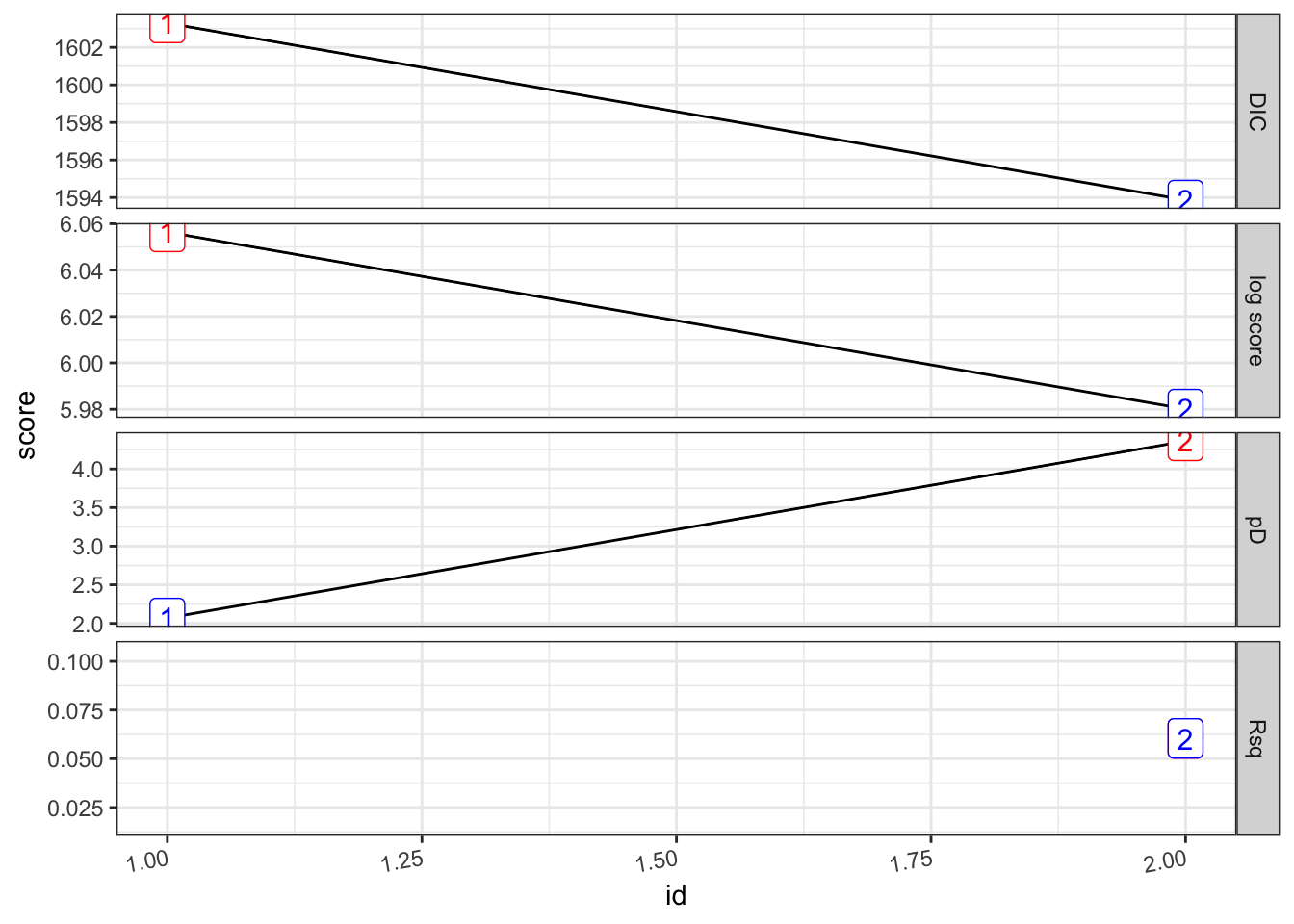
(pv_22.s <- test_pv_22 %>%
  purrr::map(~Rsq.batch.safe(model = ., dic.null = test_pv_22[[1]]$dic, n = n2)) %>%
  bind_rows(.id = "formula") %>% mutate(id = row_number()))

pv_22.s %>%
  plot_score()

# Sumamry
summary(test_pv_22[[2]])

## 
## Call:
##    c("inla(formula = formula, family = \"nbinomial\", data = dat1, offset 
##    = log(pob), ", " verbose = F, control.compute = list(config = T, dic = 
##    T, ", " cpo = T, waic = T), control.predictor = list(link = 1, ", " 
##    compute = TRUE), control.fixed = list(correlation.matrix = T))" ) 
## Time used:
##     Pre = 1.3, Running = 0.493, Post = 0.235, Total = 2.03 
## Fixed effects:
##               mean    sd 0.025quant 0.5quant 0.975quant   mode kld
## (Intercept) -5.107 0.706     -6.539   -5.103     -3.698 -5.096   0
## viirs       -0.461 0.249     -0.956   -0.461      0.034 -0.461   0
## 
## Linear combinations (derived):
##             ID   mean    sd 0.025quant 0.5quant 0.975quant   mode kld
## (Intercept)  1 -5.107 0.706     -6.539   -5.103     -3.698 -5.097   0
## viirs        2 -0.461 0.249     -0.963   -0.458      0.026 -0.453   0
## 
## Random effects:
##   Name     Model
##     index BYM model
##    year IID model
## 
## Model hyperparameters:
##                                                            mean       sd
## size for the nbinomial observations (1/overdispersion)    1.390    0.273
## Precision for index (iid component)                    1890.151 1876.880
## Precision for index (spatial component)                   0.225    0.113
## Precision for year                                        0.856    0.599
##                                                        0.025quant 0.5quant
## size for the nbinomial observations (1/overdispersion)      0.923    1.367
## Precision for index (iid component)                       128.527 1335.227
## Precision for index (spatial component)                     0.079    0.202
## Precision for year                                          0.165    0.711
##                                                        0.975quant    mode
## size for the nbinomial observations (1/overdispersion)       1.99   1.324
## Precision for index (iid component)                       6863.22 351.987
## Precision for index (spatial component)                      0.51   0.161
## Precision for year                                           2.40   0.439
## 
## Expected number of effective parameters(stdev): 16.12(0.834)
## Number of equivalent replicates : 3.72 
## 
## Deviance Information Criterion (DIC) ...............: 746.60
## Deviance Information Criterion (DIC, saturated) ....: 92.30
## Effective number of parameters .....................: 17.13
## 
## Watanabe-Akaike information criterion (WAIC) ...: 747.21
## Effective number of parameters .................: 14.67
## 
## Marginal log-Likelihood:  -410.29 
## CPO and PIT are computed
## 
## Posterior marginals for the linear predictor and
##  the fitted values are computed

summary(test_pv_22[[3]])

## 
## Call:
##    c("inla(formula = formula, family = \"nbinomial\", data = dat1, offset 
##    = log(pob), ", " verbose = F, control.compute = list(config = T, dic = 
##    T, ", " cpo = T, waic = T), control.predictor = list(link = 1, ", " 
##    compute = TRUE), control.fixed = list(correlation.matrix = T))" ) 
## Time used:
##     Pre = 1.39, Running = 0.586, Post = 0.343, Total = 2.32 
## Fixed effects:
##               mean   sd 0.025quant 0.5quant 0.975quant   mode kld
## (Intercept) -5.569 0.68     -6.937   -5.568     -4.207 -5.567   0
## 
## Linear combinations (derived):
##             ID   mean   sd 0.025quant 0.5quant 0.975quant   mode kld
## (Intercept)  1 -5.569 0.68     -6.937   -5.568     -4.207 -5.566   0
## 
## Random effects:
##   Name     Model
##     index BYM model
##    year IID model
##    inla.group(viirs) RW1 model
## 
## Model hyperparameters:
##                                                            mean       sd
## size for the nbinomial observations (1/overdispersion) 1.38e+00 2.71e-01
## Precision for index (iid component)                    1.91e+03 1.91e+03
## Precision for index (spatial component)                1.96e-01 9.20e-02
## Precision for year                                     8.13e-01 5.67e-01
## Precision for inla.group(viirs)                        1.87e+04 1.85e+04
##                                                        0.025quant 0.5quant
## size for the nbinomial observations (1/overdispersion)      0.915 1.35e+00
## Precision for index (iid component)                       130.996 1.35e+03
## Precision for index (spatial component)                     0.073 1.78e-01
## Precision for year                                          0.157 6.76e-01
## Precision for inla.group(viirs)                          1268.790 1.33e+04
##                                                        0.975quant     mode
## size for the nbinomial observations (1/overdispersion)   1.98e+00    1.311
## Precision for index (iid component)                      6.99e+03  358.525
## Precision for index (spatial component)                  4.27e-01    0.146
## Precision for year                                       2.27e+00    0.419
## Precision for inla.group(viirs)                          6.74e+04 3466.127
## 
## Expected number of effective parameters(stdev): 16.05(0.771)
## Number of equivalent replicates : 3.74 
## 
## Deviance Information Criterion (DIC) ...............: 746.88
## Deviance Information Criterion (DIC, saturated) ....: 91.97
## Effective number of parameters .....................: 17.00
## 
## Watanabe-Akaike information criterion (WAIC) ...: 747.57
## Effective number of parameters .................: 14.61
## 
## Marginal log-Likelihood:  -413.16 
## CPO and PIT are computed
## 
## Posterior marginals for the linear predictor and
##  the fitted values are computed

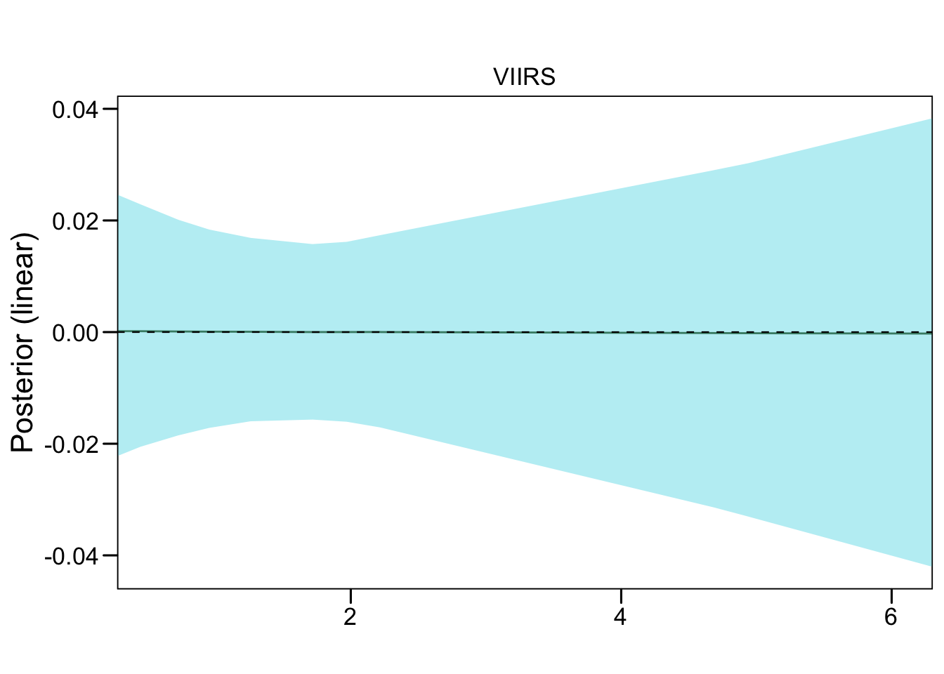
test_pv_22[[3]] %>%
  plot_random3(exp = F, lab1 = "VIIRS", vars = "inla.group(viirs)")

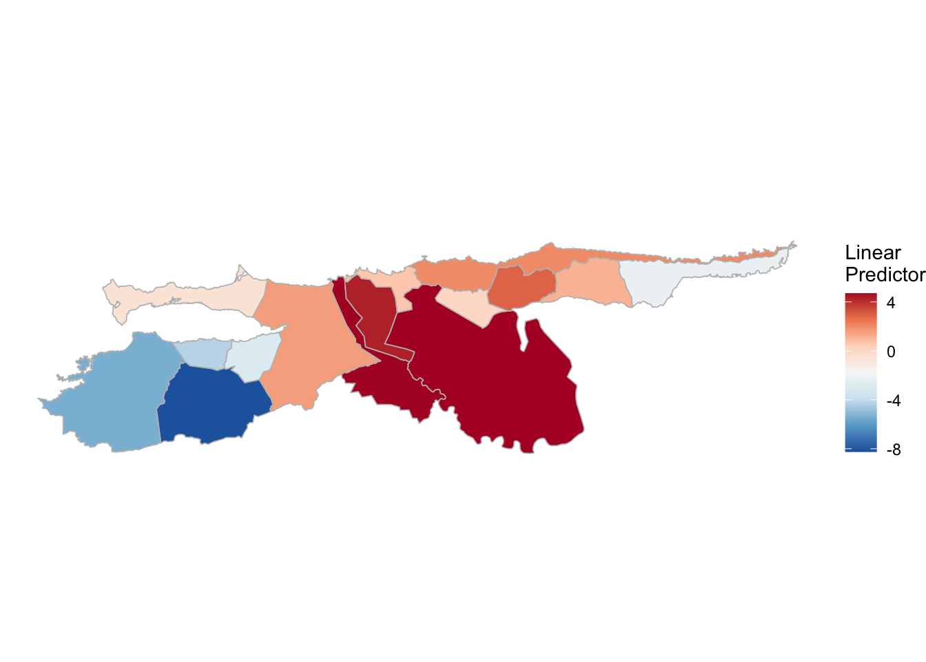
(rm_pv_1 <- test_pv_22[[2]] %>% plot_random_map2(map = vzla.sf, name= "", id = MUNICIPI0, col1 = "gray"))

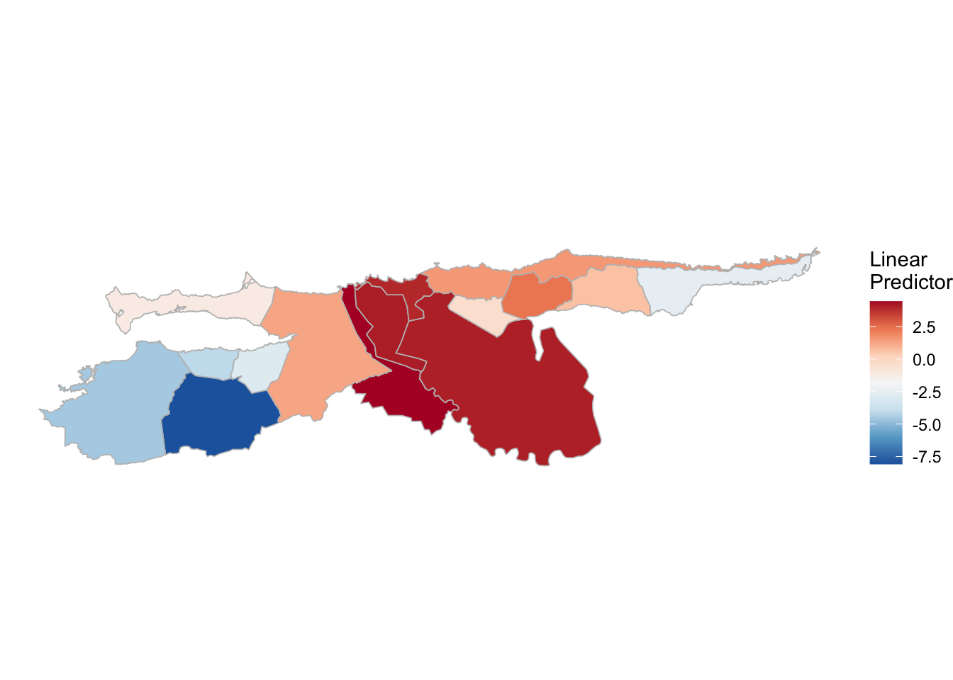
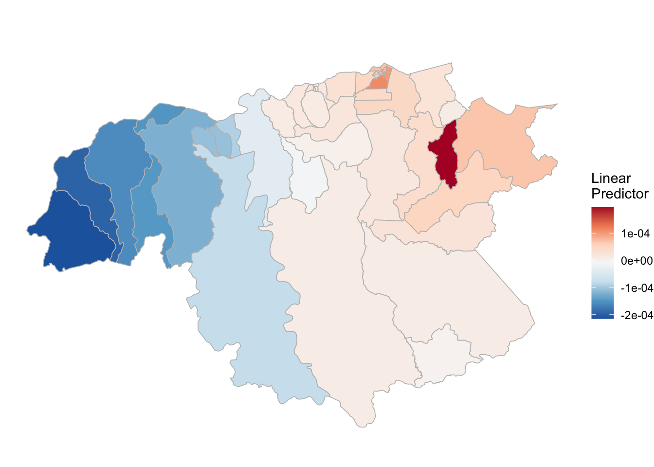
(rm_pv_2 <- test_pv_22[[3]] %>% plot_random_map2(map = vzla.sf, name= "", id = MUNICIPI0, col1 = "gray"))