Chapter 5 Sensitivity Analysis 1

5.1 Data

rm(list=ls())
library(tidyverse)
library(purrr)
library(Metrics)
library(stringr)
library(MatrixModels)
library(sf)

load("./_dat/NL_VEN_dat3.RData")

# Scaling
dt.pred <- dt_final %>%
  group_by(index) %>%
  mutate(viirs = scale_this(viirs),
         mei = scale_this(mei),
         yy = Year,
         Year = Year-2012) %>% #start year on 2012
  ungroup() %>%
  nest(data = everything()) %>%
  crossing(yy=2013:2015) %>%
  mutate(dat_subset = purrr::map2(.x = data, .y = yy, .f = ~mutate(.x, PV = ifelse(yy>.y,NA,PV),
                                                                   PF = ifelse(yy>.y,NA,PF))))

5.2 Municipios with no mining

5.2.1 Functions

library(INLA)
library(spdep)
library(purrr)
devtools::source_gist("https://gist.github.com/gcarrascoe/89e018d99bad7d3365ec4ac18e3817bd")

inla.batch <- function(formula, dat1 = dt_final1) {
  result = inla(formula, data=dat1, family="nbinomial", offset=log(pop), verbose = F, 
                #control.inla=list(strategy="gaussian"),
                control.compute=list(config=T, dic=T, cpo=T, waic=T),
                control.fixed = list(correlation.matrix=T),
                control.predictor=list(link=1,compute=TRUE)
                )
  return(result)
}

inla.batch.safe <- possibly(inla.batch, otherwise = NA_real_)

5.3 Subset

area.bs1 <- area.bs %>%
  mutate(ii = ifelse(cod == "SIFONTES-DALLA COSTA", 1, 0),
         ii = ifelse(cod == "SIFONTES-SAN ISIDRO", 1, ii)) %>%
  filter(ii!=1)

5.3.1 P. vivax

#Create adjacency matrix
n1 <- nrow(dt_final1)
nb.map1 <- poly2nb(area.bs1)
nb2INLA("./map1.graph",nb.map1)

codes1<-as.data.frame(area.bs1)
codes1$index<-as.numeric(row.names(codes1))
codes1<-subset(codes1,select=c("cod","index"))
dt_final1<-merge(d_v_yy,codes1,by="cod") %>%
    mutate(ii = ifelse(cod == "SIFONTES-DALLA COSTA", 1, 0),
         ii = ifelse(cod == "SIFONTES-SAN ISIDRO", 1, ii)) %>%
  filter(ii!=1)

# MODEL
pv_21<-c(formula = PV ~ 1,
        formula = PV ~ 1 + f(index, model = "bym", graph = "./map1.graph") + 
          f(Year, model = "iid") + viirs + mei,
        formula = PV ~ 1 + f(index, model = "bym", graph = "./map1.graph") + 
          f(Year, model = "iid") + f(inla.group(viirs), model = "rw1") + mei)

# ------------------------------------------
# PV estimation
# ------------------------------------------
names(pv_21)<-pv_21

INLA:::inla.dynload.workaround()
test_pv_21 <- pv_21 %>% purrr::map(~inla.batch.safe(formula = .))

(pv_21.s <- test_pv_21 %>%
  purrr::map(~Rsq.batch.safe(model = ., dic.null = test_pv_21[[1]]$dic, n = n1)) %>%
  bind_rows(.id = "formula") %>% mutate(id = row_number()))

pv_21.s %>%
  plot_score()

# Sumamry
summary(test_pv_21[[2]])

## 
## Call:
##    c("inla(formula = formula, family = \"nbinomial\", data = dat1, offset 
##    = log(pop), ", " verbose = F, control.compute = list(config = T, dic = 
##    T, ", " cpo = T, waic = T), control.predictor = list(link = 1, ", " 
##    compute = TRUE), control.fixed = list(correlation.matrix = T))" ) 
## Time used:
##     Pre = 1.07, Running = 1.89, Post = 0.271, Total = 3.22 
## Fixed effects:
##               mean    sd 0.025quant 0.5quant 0.975quant   mode kld
## (Intercept) -4.981 0.461     -5.868   -4.994     -4.023 -5.017   0
## viirs       -0.270 0.018     -0.305   -0.270     -0.236 -0.269   0
## mei         -0.970 0.275     -1.483   -0.980     -0.399 -0.999   0
## 
## Linear combinations (derived):
##             ID   mean    sd 0.025quant 0.5quant 0.975quant   mode kld
## (Intercept)  1 -4.981 0.461     -5.876   -4.991     -4.029 -5.006   0
## viirs        2 -0.270 0.018     -0.305   -0.270     -0.236 -0.269   0
## mei          3 -0.970 0.276     -1.512   -0.970     -0.429 -0.969   0
## 
## Random effects:
##   Name     Model
##     index BYM model
##    Year IID model
## 
## Model hyperparameters:
##                                                            mean       sd
## size for the nbinomial observations (1/overdispersion)    0.203    0.018
## Precision for index (iid component)                    1753.521 1780.363
## Precision for index (spatial component)                1723.368 1741.564
## Precision for Year                                        2.502    2.366
##                                                        0.025quant 0.5quant
## size for the nbinomial observations (1/overdispersion)      0.169    0.203
## Precision for index (iid component)                        99.900 1215.408
## Precision for index (spatial component)                   100.544 1198.720
## Precision for Year                                          0.371    1.819
##                                                        0.975quant    mode
## size for the nbinomial observations (1/overdispersion)      0.242   0.202
## Precision for index (iid component)                      6516.131 257.846
## Precision for index (spatial component)                  6387.709 263.147
## Precision for Year                                          8.736   0.951
## 
## Expected number of effective parameters(stdev): 6.16(0.528)
## Number of equivalent replicates : 34.90 
## 
## Deviance Information Criterion (DIC) ...............: 2153.24
## Deviance Information Criterion (DIC, saturated) ....: NaN
## Effective number of parameters .....................: 7.38
## 
## Watanabe-Akaike information criterion (WAIC) ...: 2154.65
## Effective number of parameters .................: 7.57
## 
## Marginal log-Likelihood:  -1102.11 
## CPO and PIT are computed
## 
## Posterior marginals for the linear predictor and
##  the fitted values are computed

summary(test_pv_21[[3]])

## 
## Call:
##    c("inla(formula = formula, family = \"nbinomial\", data = dat1, offset 
##    = log(pop), ", " verbose = F, control.compute = list(config = T, dic = 
##    T, ", " cpo = T, waic = T), control.predictor = list(link = 1, ", " 
##    compute = TRUE), control.fixed = list(correlation.matrix = T))" ) 
## Time used:
##     Pre = 1.2, Running = 2.25, Post = 0.234, Total = 3.69 
## Fixed effects:
##                mean    sd 0.025quant 0.5quant 0.975quant    mode kld
## (Intercept) -13.195 1.120    -15.414  -13.194    -10.989 -13.190   0
## mei          -0.446 0.517     -1.460   -0.447      0.573  -0.449   0
## 
## Linear combinations (derived):
##             ID    mean    sd 0.025quant 0.5quant 0.975quant    mode kld
## (Intercept)  1 -13.196 1.120    -15.410  -13.196    -10.988 -13.194   0
## mei          2  -0.446 0.517     -1.461   -0.446      0.572  -0.447   0
## 
## Random effects:
##   Name     Model
##     index BYM model
##    Year IID model
##    inla.group(viirs) RW1 model
## 
## Model hyperparameters:
##                                                            mean       sd
## size for the nbinomial observations (1/overdispersion)    0.938    0.123
## Precision for index (iid component)                       0.123    0.031
## Precision for index (spatial component)                1812.361 1745.562
## Precision for Year                                        0.667    0.424
## Precision for inla.group(viirs)                           2.899    1.875
##                                                        0.025quant 0.5quant
## size for the nbinomial observations (1/overdispersion)      0.717    0.930
## Precision for index (iid component)                         0.072    0.119
## Precision for index (spatial component)                   118.635 1299.631
## Precision for Year                                          0.164    0.568
## Precision for inla.group(viirs)                             0.745    2.438
##                                                        0.975quant    mode
## size for the nbinomial observations (1/overdispersion)      1.201   0.917
## Precision for index (iid component)                         0.194   0.113
## Precision for index (spatial component)                  6411.274 321.702
## Precision for Year                                          1.764   0.395
## Precision for inla.group(viirs)                             7.789   1.713
## 
## Expected number of effective parameters(stdev): 51.45(1.65)
## Number of equivalent replicates : 4.18 
## 
## Deviance Information Criterion (DIC) ...............: 1889.96
## Deviance Information Criterion (DIC, saturated) ....: NaN
## Effective number of parameters .....................: 51.21
## 
## Watanabe-Akaike information criterion (WAIC) ...: 1886.26
## Effective number of parameters .................: 38.29
## 
## Marginal log-Likelihood:  -1025.01 
## CPO and PIT are computed
## 
## Posterior marginals for the linear predictor and
##  the fitted values are computed

test_pv_21[[3]] %>%
  plot_random3(exp = F, lab1 = "VIIRS", vars = "inla.group(viirs)")

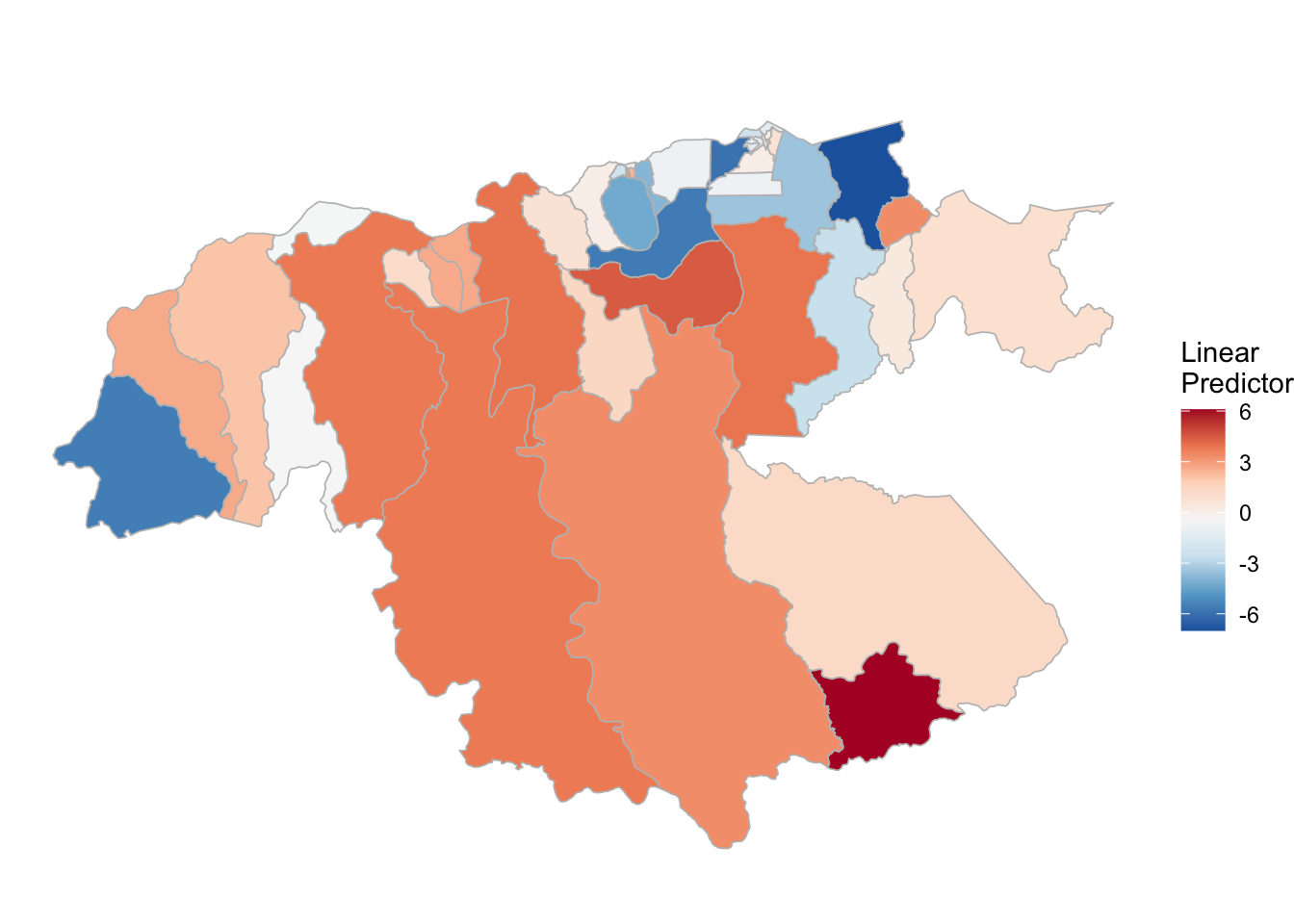
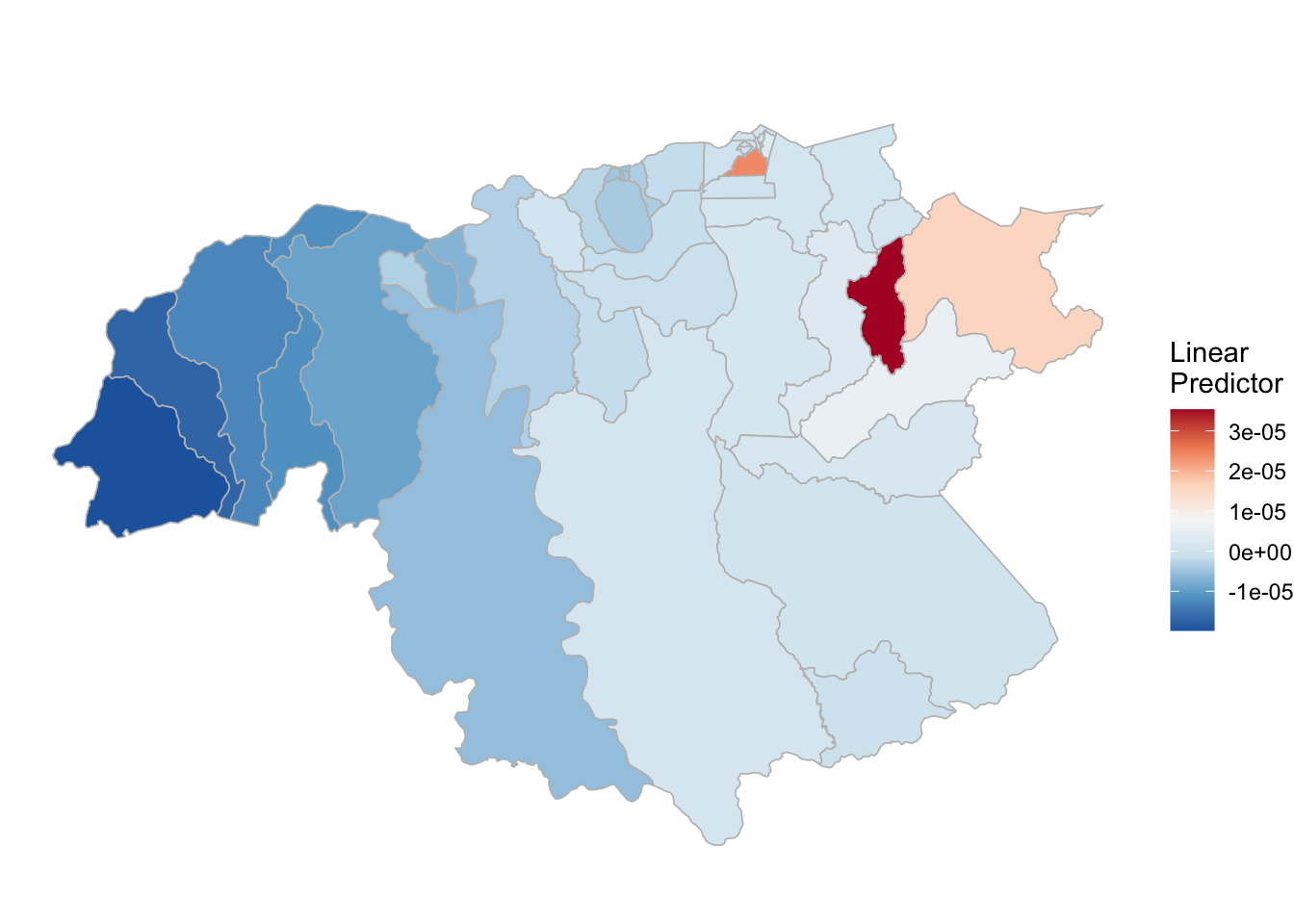
(rm_pv_1 <- test_pv_21[[2]] %>% plot_random_map2(map = area.bs1, name= "", id = cod, col1 = "gray"))

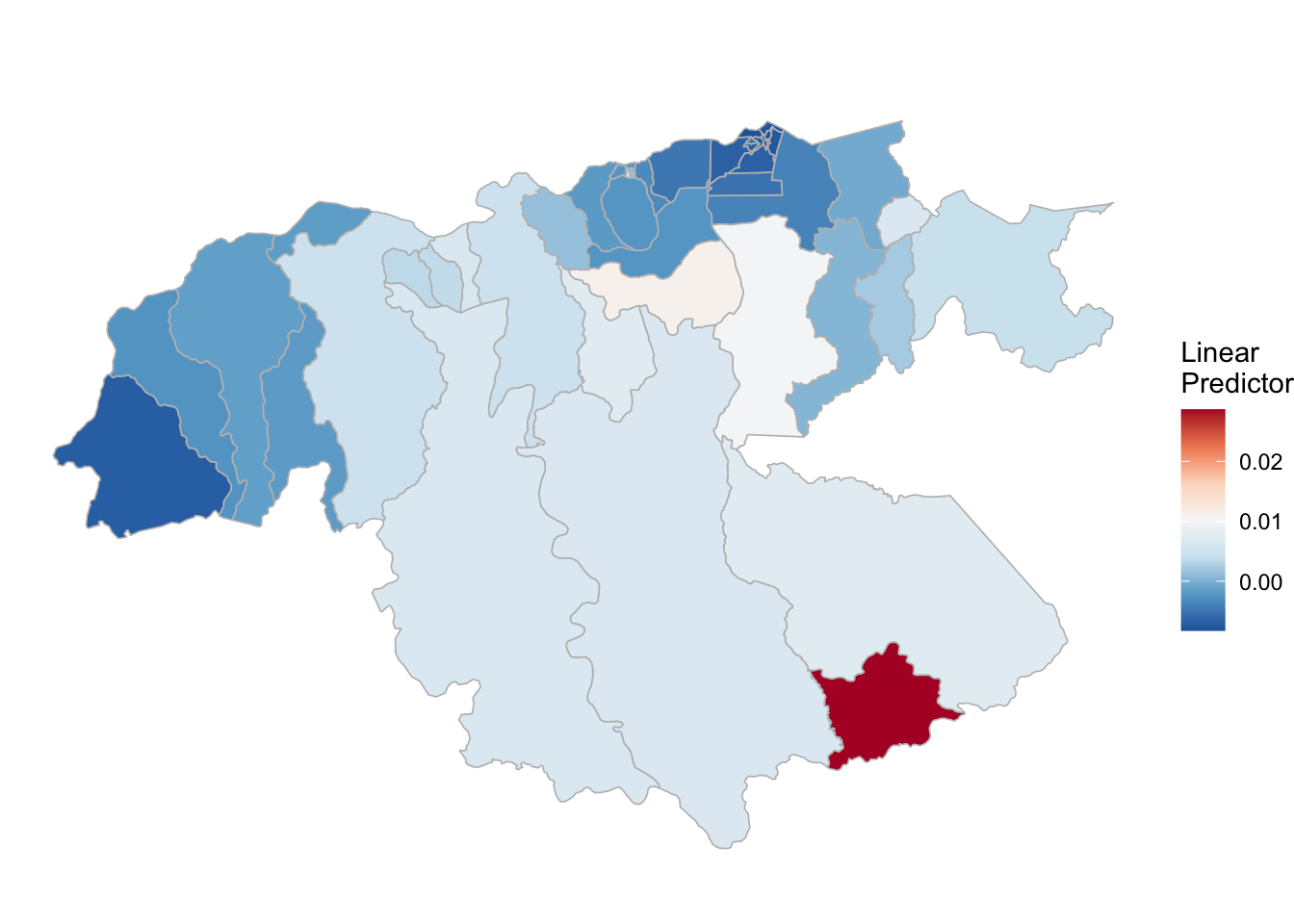
(rm_pv_2 <- test_pv_21[[3]] %>% plot_random_map2(map = area.bs1, name= "", id = cod, col1 = "gray"))

5.3.2 P. falciparum

# MODEL
pf_21<-c(formula = PF ~ 1,
        formula = PF ~ 1 + f(index, model = "bym", graph = "./map1.graph") + 
          f(Year, model = "iid") + viirs + mei,
        formula = PF ~ 1 + f(index, model = "bym", graph = "./map1.graph") + 
          f(Year, model = "iid") + f(inla.group(viirs), model = "rw1") + mei)

# ------------------------------------------
# PV estimation
# ------------------------------------------
names(pf_21)<-pf_21

INLA:::inla.dynload.workaround()
test_pf_21 <- pf_21 %>% purrr::map(~inla.batch.safe(formula = .))

(pf_21.s <- test_pf_21 %>%
  purrr::map(~Rsq.batch.safe(model = ., dic.null = test_pf_21[[1]]$dic, n = n1)) %>%
  bind_rows(.id = "formula") %>% mutate(id = row_number()))

pf_21.s %>%
  plot_score()

# Sumamry
summary(test_pf_21[[2]])

## 
## Call:
##    c("inla(formula = formula, family = \"nbinomial\", data = dat1, offset 
##    = log(pop), ", " verbose = F, control.compute = list(config = T, dic = 
##    T, ", " cpo = T, waic = T), control.predictor = list(link = 1, ", " 
##    compute = TRUE), control.fixed = list(correlation.matrix = T))" ) 
## Time used:
##     Pre = 1.1, Running = 9.99, Post = 0.223, Total = 11.3 
## Fixed effects:
##               mean    sd 0.025quant 0.5quant 0.975quant   mode kld
## (Intercept) -1.650 0.443     -2.518   -1.651     -0.781 -1.651   0
## viirs       -0.040 0.030     -0.099   -0.040      0.018 -0.040   0
## mei         -0.918 0.440     -1.748   -0.930     -0.020 -0.955   0
## 
## Linear combinations (derived):
##             ID   mean    sd 0.025quant 0.5quant 0.975quant   mode kld
## (Intercept)  1 -1.650 0.443     -2.519    -1.65     -0.782 -1.650   0
## viirs        2 -0.040 0.030     -0.099    -0.04      0.018 -0.040   0
## mei          3 -0.918 0.440     -1.778    -0.92     -0.050 -0.924   0
## 
## Random effects:
##   Name     Model
##     index BYM model
##    Year IID model
## 
## Model hyperparameters:
##                                                            mean       sd
## size for the nbinomial observations (1/overdispersion) 6.80e-02 7.00e-03
## Precision for index (iid component)                    1.94e+03 1.91e+03
## Precision for index (spatial component)                1.46e+03 1.78e+03
## Precision for Year                                     1.80e+04 1.87e+04
##                                                        0.025quant 0.5quant
## size for the nbinomial observations (1/overdispersion)      0.055 6.80e-02
## Precision for index (iid component)                       132.436 1.38e+03
## Precision for index (spatial component)                    89.860 9.17e+02
## Precision for Year                                       1255.251 1.24e+04
##                                                        0.975quant     mode
## size for the nbinomial observations (1/overdispersion)   8.20e-02    0.069
## Precision for index (iid component)                      7.00e+03  360.880
## Precision for index (spatial component)                  6.19e+03  241.454
## Precision for Year                                       6.80e+04 3444.573
## 
## Expected number of effective parameters(stdev): 3.01(0.015)
## Number of equivalent replicates : 71.33 
## 
## Deviance Information Criterion (DIC) ...............: 1802.65
## Deviance Information Criterion (DIC, saturated) ....: NaN
## Effective number of parameters .....................: -0.172
## 
## Watanabe-Akaike information criterion (WAIC) ...: 1804.16
## Effective number of parameters .................: 1.32
## 
## Marginal log-Likelihood:  -950.82 
## CPO and PIT are computed
## 
## Posterior marginals for the linear predictor and
##  the fitted values are computed

summary(test_pf_21[[3]])

## 
## Call:
##    c("inla(formula = formula, family = \"nbinomial\", data = dat1, offset 
##    = log(pop), ", " verbose = F, control.compute = list(config = T, dic = 
##    T, ", " cpo = T, waic = T), control.predictor = list(link = 1, ", " 
##    compute = TRUE), control.fixed = list(correlation.matrix = T))" ) 
## Time used:
##     Pre = 1.24, Running = 4.71, Post = 0.217, Total = 6.17 
## Fixed effects:
##                mean    sd 0.025quant 0.5quant 0.975quant    mode kld
## (Intercept) -15.991 1.187    -18.373  -15.975    -13.686 -15.937   0
## mei           0.608 0.593     -0.588    0.620      1.741   0.642   0
## 
## Linear combinations (derived):
##             ID    mean    sd 0.025quant 0.5quant 0.975quant    mode kld
## (Intercept)  1 -15.991 1.186    -18.349  -15.983    -13.666 -15.961   0
## mei          2   0.609 0.594     -0.552    0.607      1.778   0.604   0
## 
## Random effects:
##   Name     Model
##     index BYM model
##    Year IID model
##    inla.group(viirs) RW1 model
## 
## Model hyperparameters:
##                                                            mean       sd
## size for the nbinomial observations (1/overdispersion)    1.238    0.346
## Precision for index (iid component)                       0.118    0.025
## Precision for index (spatial component)                1650.189 1816.043
## Precision for Year                                        0.633    0.656
## Precision for inla.group(viirs)                           2.668    1.899
##                                                        0.025quant 0.5quant
## size for the nbinomial observations (1/overdispersion)      0.815    1.154
## Precision for index (iid component)                         0.073    0.116
## Precision for index (spatial component)                   111.319 1100.339
## Precision for Year                                          0.009    0.394
## Precision for inla.group(viirs)                             0.579    2.185
##                                                        0.975quant    mode
## size for the nbinomial observations (1/overdispersion)      2.122   0.973
## Precision for index (iid component)                         0.171   0.115
## Precision for index (spatial component)                  6508.760 301.667
## Precision for Year                                          2.305   0.007
## Precision for inla.group(viirs)                             7.634   1.418
## 
## Expected number of effective parameters(stdev): 48.14(1.06)
## Number of equivalent replicates : 4.47 
## 
## Deviance Information Criterion (DIC) ...............: 1343.98
## Deviance Information Criterion (DIC, saturated) ....: NaN
## Effective number of parameters .....................: 45.91
## 
## Watanabe-Akaike information criterion (WAIC) ...: 1336.63
## Effective number of parameters .................: 31.19
## 
## Marginal log-Likelihood:  -749.02 
## CPO and PIT are computed
## 
## Posterior marginals for the linear predictor and
##  the fitted values are computed

test_pf_21[[3]] %>%
  plot_random3(exp = F, lab1 = "VIIRS", vars = "inla.group(viirs)")

(rm_pf_1 <- test_pf_21[[2]] %>% plot_random_map2(map = area.bs1, name= "", id = cod, col1 = "gray"))

(rm_pf_2 <- test_pf_21[[3]] %>% plot_random_map2(map = area.bs1, name= "", id = cod, col1 = "gray"))