Chapter 2 Exploratory Analysis
rm(list=ls())
library(tidyverse)
library(sf)
library(readxl)
library(stringr)
library(ggthemes)
library(ggExtra)
library(colorspace)

load("./_dat/NL_VEN_dat.RData")

map<-readRDS("./_dat/nl_ven.rds")

viirs <- map %>%
  st_set_geometry(NULL) %>%
  gather(time, viirs, X20120401:X20191201) %>%
  mutate(Year = as.numeric(str_sub(time,2,5)),
         Month = as.numeric(str_sub(time,6,7)))

dat <- read_excel("./_dat/Malaria_Data_Southern_Venezuela_1996-2016.xlsx") %>%
  dplyr::rename(ADM3_ES = Parroquia, ADM2_ES = Municipio) %>%
  mutate(ADM3_ES = str_replace(ADM3_ES, "S\\.C\\.", "SECCION CAPITAL"),
         ADM3_ES = str_replace(ADM3_ES, "A\\.E\\. ", "ANDRES ELOY "),
         ADM3_ES = str_replace(ADM3_ES, "C\\. P\\. P\\.", "CAPITAL PADRE PEDRO"),
         ADM3_ES = str_replace(ADM3_ES, "CEDEñO","CEDEÑO"),
         ADM3_ES = str_replace(ADM3_ES, "SABANA","SABAN"),
         ADM3_ES = str_replace(ADM3_ES, "C\\.","CAPITAL"),
         ADM2_ES = str_replace(ADM2_ES, "CEDEñO","CEDEÑO"),
         ADM2_ES = str_replace(ADM2_ES, "Heres","HERES")) %>%
  filter(ADM3_ES!="CINCO DE JULIO") %>%
  filter(ADM3_ES!="SALOM")

# mei <- mei %>%
#   rename(Year = year)

d <- dat %>%
  inner_join(viirs, by = c("ADM2_ES", "ADM3_ES","Year","Month")) %>%
  inner_join(mei, by = c("ADM2_ES", "ADM3_ES","Year"))

#save.image("./_dat/NL_VEN_dat.RData")
#write.csv(d_v_yy, "./_dat/dat_ven.csv", na="", row.names = F)
2.1 TIME SERIES
2.1.1 Bolivar state
source("./_dat/nl_functions.R")

d_yy %>%
  dual_plot(x = Year, y_left = r.pv, y_right = viirs,
            y2_left = "r.pf",
             col_right = "#69b3a2", col_left = "#CD3700",
             labels_legend = c("P.vivax","P.falciparum"), name_legend = "Malaria rate: ") +
  labs(y= "Malaria rate")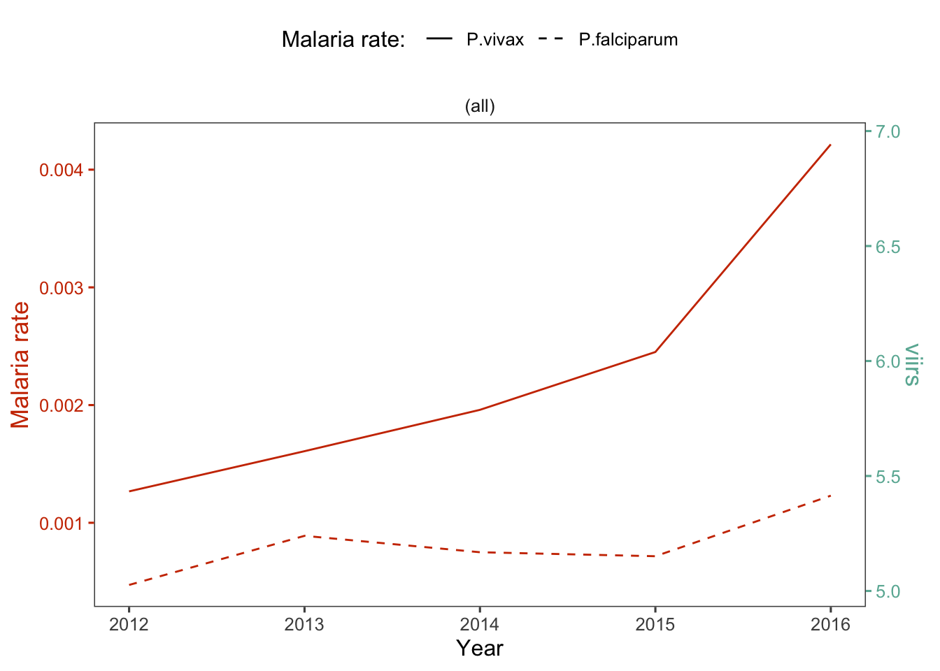
d_yy %>%
  var_plot()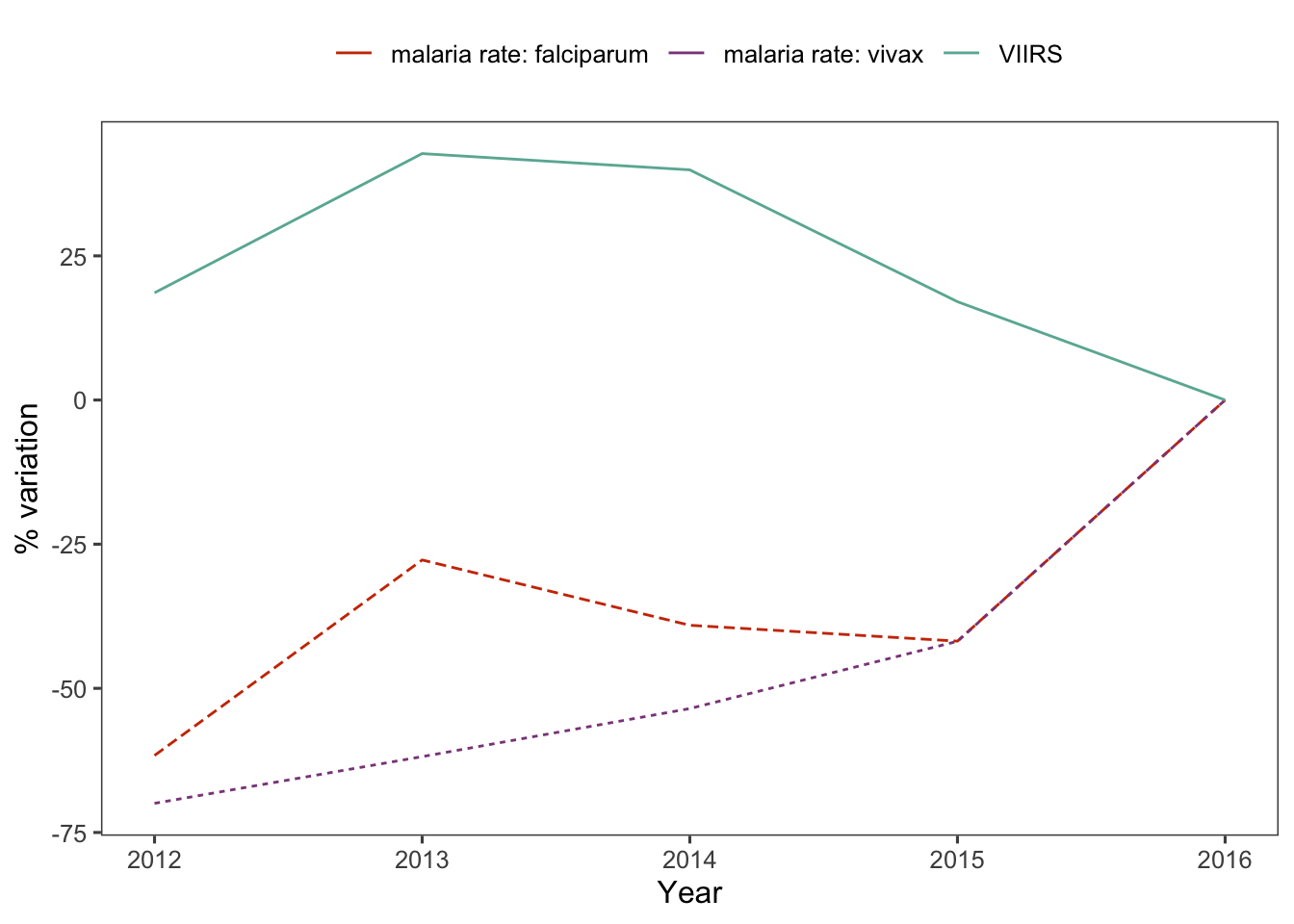
2.1.2 Municipality
d_m_yy %>%
  dual_plot(x = Year, y_left = r.pv, y_right = viirs, group="ADM2_ES", y2_left = "r.pf",
             col_right = "#69b3a2", col_left = "#CD3700",
             labels_legend = c("P.vivax","P.falciparum"), name_legend = "Malaria rate: ") +
  labs(y= "Malaria rate")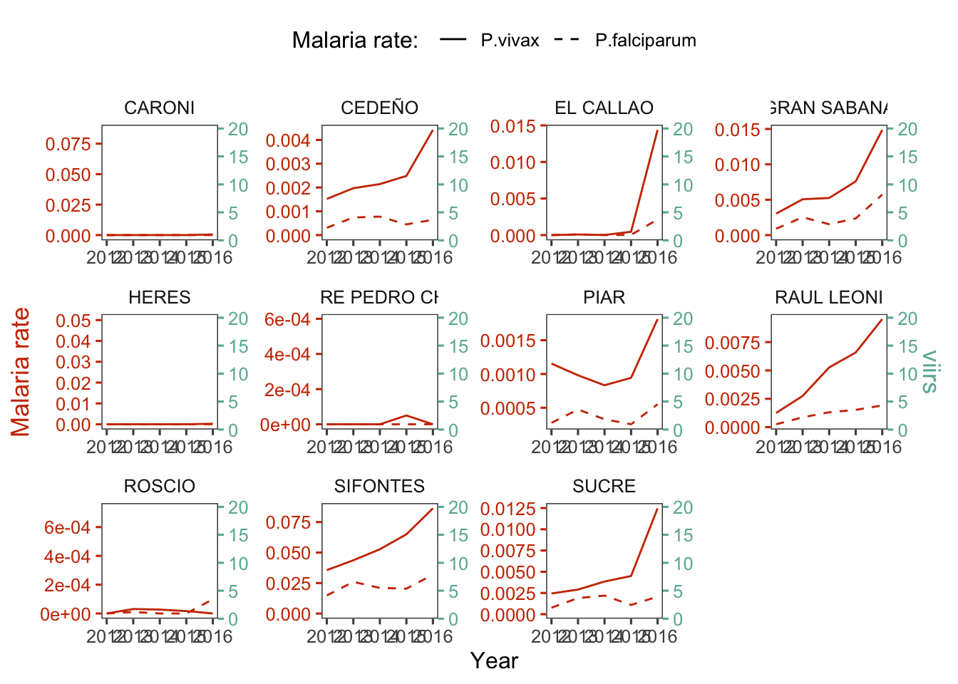
d_m_yy %>%
  group_by(ADM2_ES) %>%
  var_plot(group = "ADM2_ES") +
  facet_wrap(~ADM2_ES, scales = "free")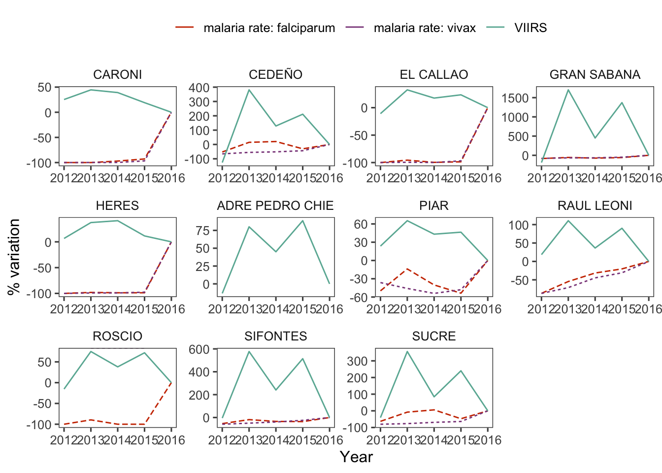
2.1.3 Parish
d_v_yy %>%
  mutate(r.pv = r.pv*1000,
         r.pf = r.pf*1000) %>%
  dual_plot(x = Year, y_left = r.pv, y_right = viirs, group="cod", y2_left = "r.pf",
             col_right = "#69b3a2", col_left = "#CD3700",
             labels_legend = c("P.vivax","P.falciparum"), name_legend = "Malaria rate: ") +
  labs(y= "Malaria rate (x. 1000 hab.)")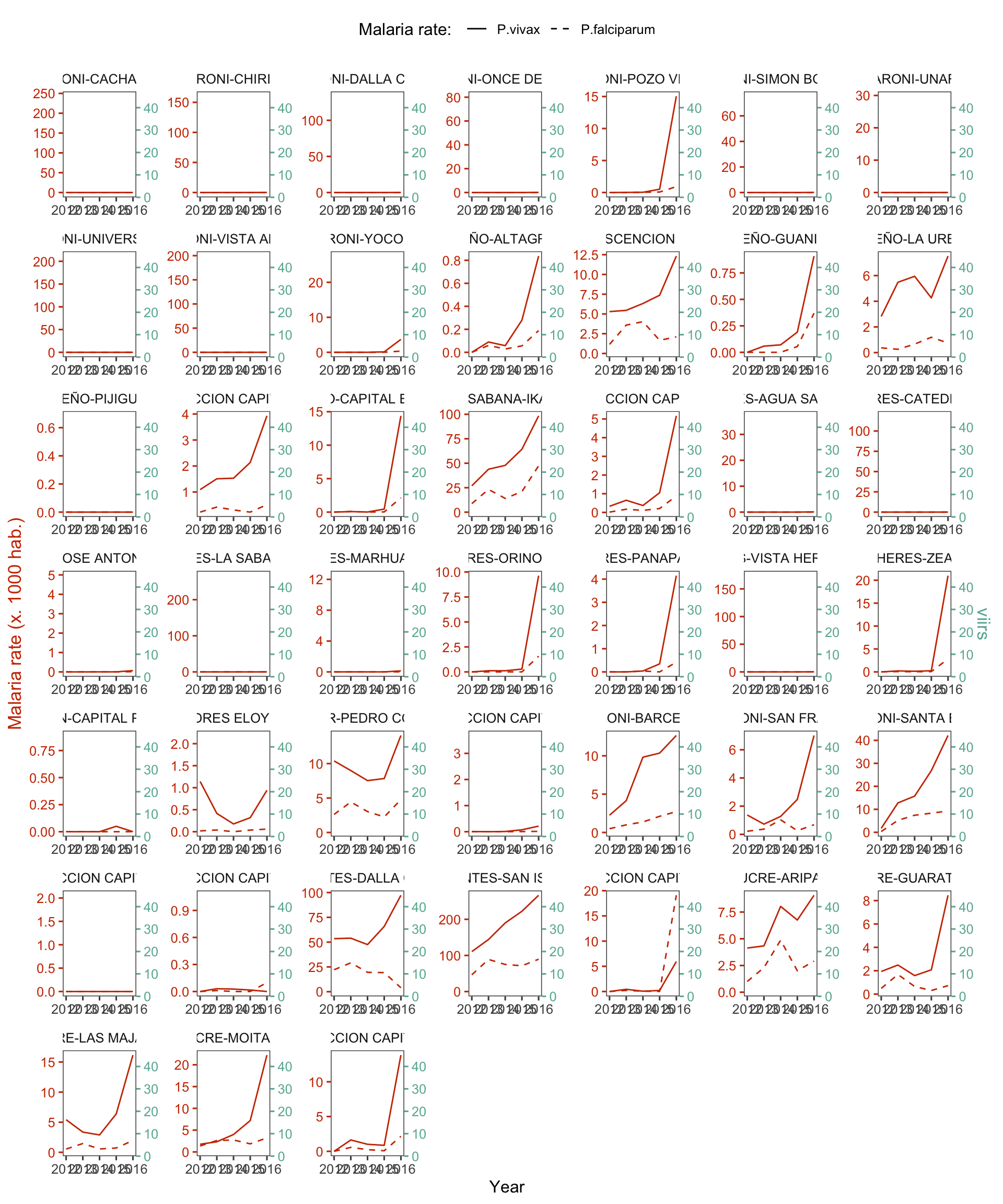
d_v_yy %>%
  group_by(cod) %>%
  var_plot(group = "cod") +
  facet_wrap(~cod, scales = "free")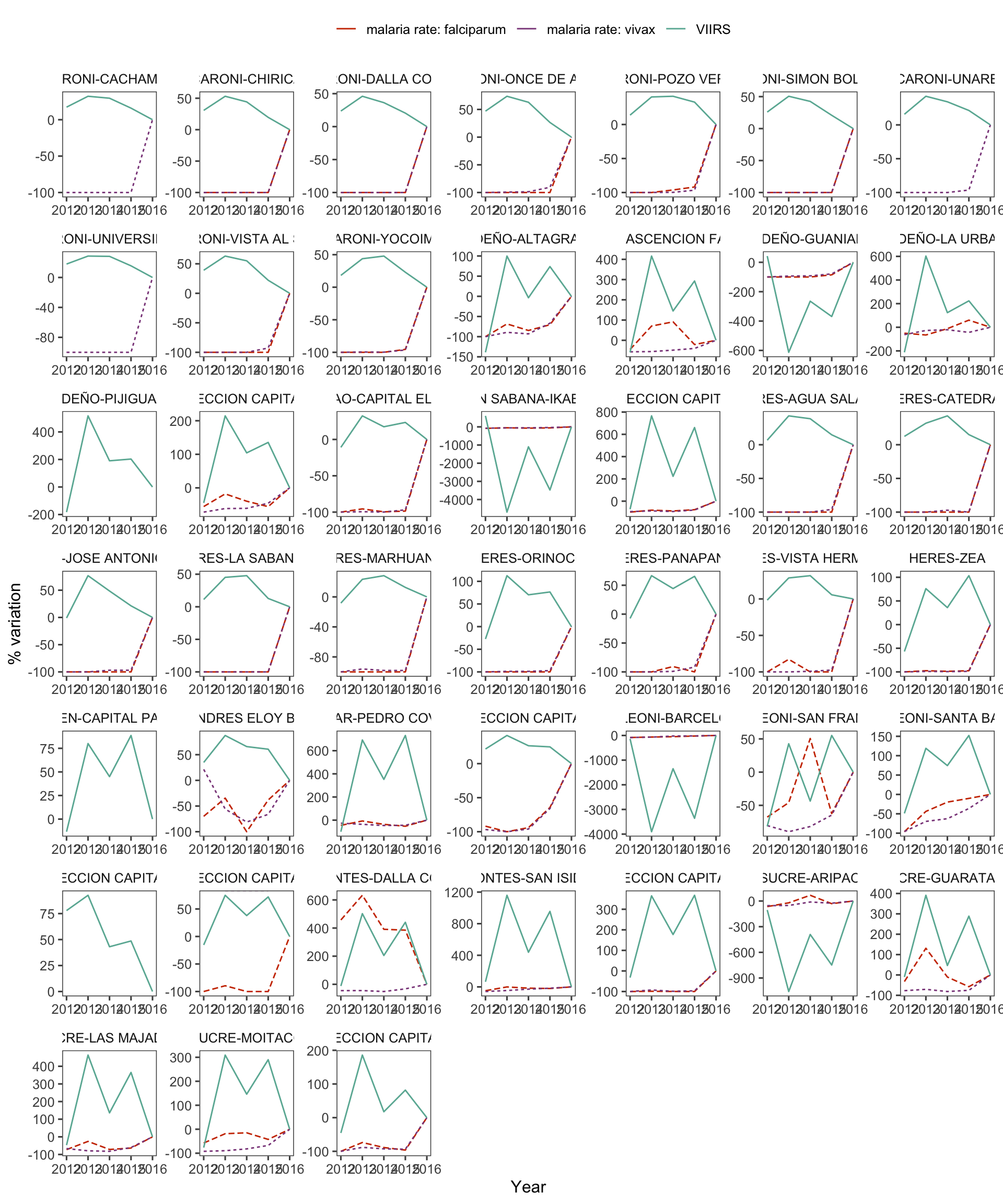
2.2 VIIRS-MALARIA FUNCTION
2.2.1 Bolivar state
d_yy %>%
  mutate(r.pv = r.pv*1000,
         r.pf = r.pf*1000) %>%
  dplyr::select(r.pv, r.pf, viirs) %>%
  gather(type, rate, r.pv:r.pf) %>%
  bi_plot()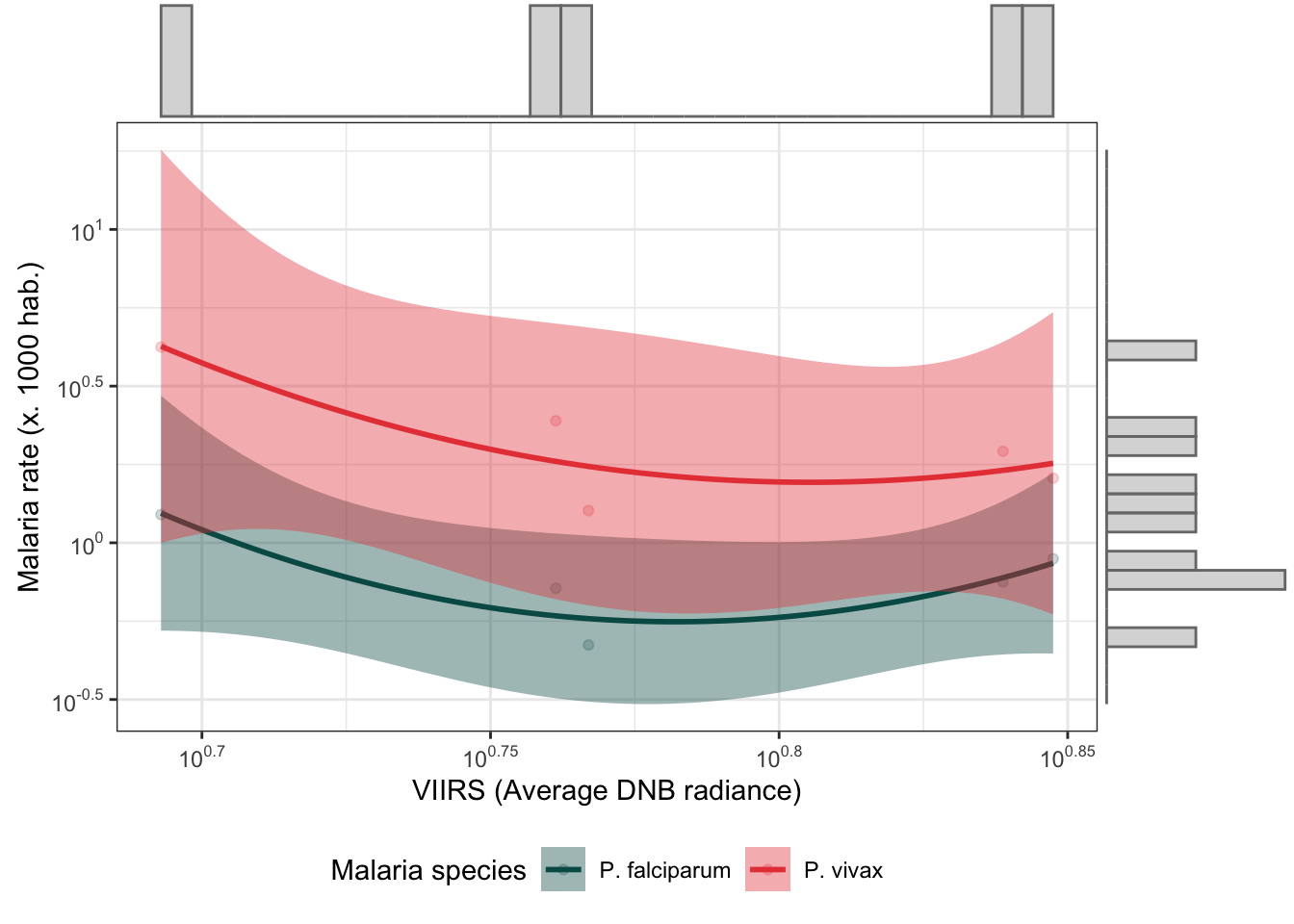
d_yy %>%
  mutate(r.pv = r.pv*1000,
         r.pf = r.pf*1000) %>%
  dplyr::select(r.pv, r.pf, viirs) %>%
  gather(type, rate, r.pv:r.pf) %>%
  bi_plot(trans_x = F)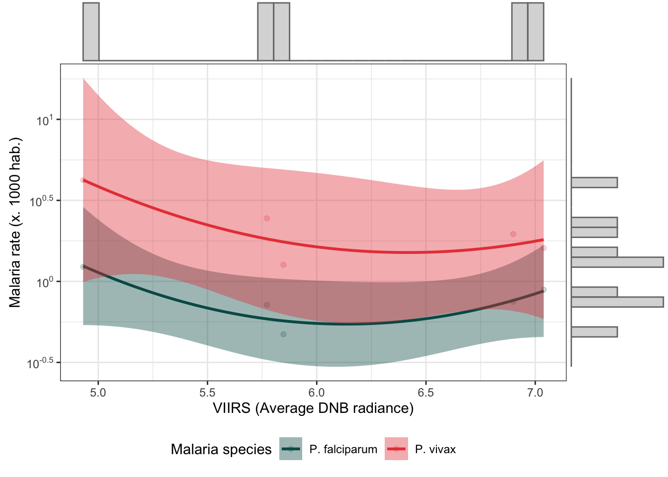
2.2.2 Municipality
d_m_yy %>%
  mutate(r.pv = r.pv*1000,
         r.pf = r.pf*1000) %>%
  dplyr::select(r.pv, r.pf, ADM2_ES, viirs) %>%
  gather(type, rate, r.pv:r.pf) %>%
  bi_plot()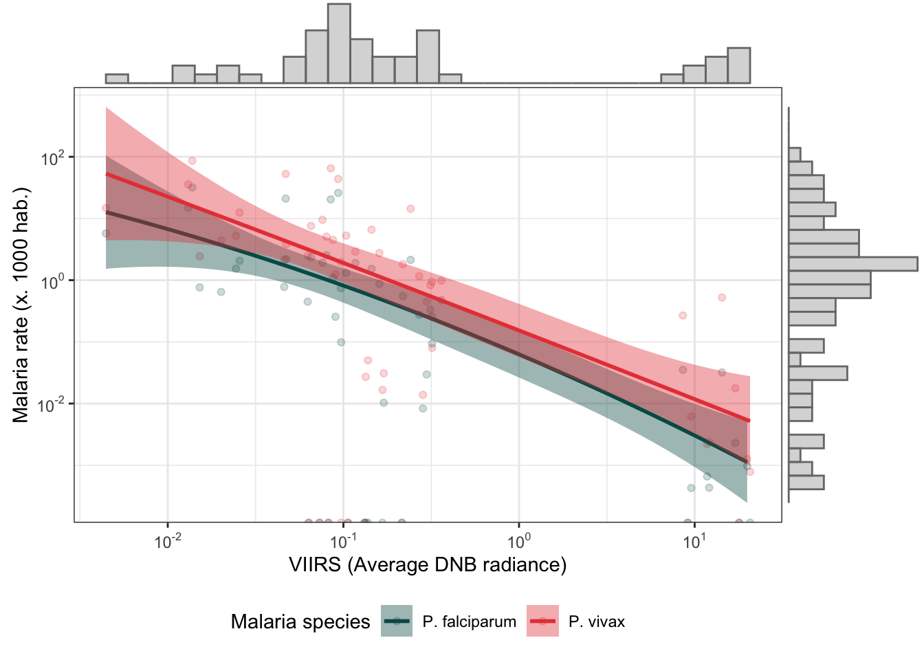
d_m_yy %>%
  mutate(r.pv = r.pv*1000,
         r.pf = r.pf*1000) %>%
  dplyr::select(r.pv, r.pf, ADM2_ES, viirs) %>%
  gather(type, rate, r.pv:r.pf) %>%
  bi_plot(trans_x = F)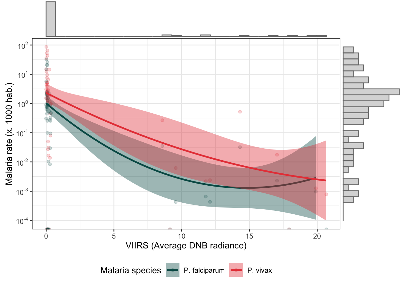
2.2.3 Parish
d_v_yy %>%
  mutate(r.pv = r.pv*1000,
         r.pf = r.pf*1000) %>%
  dplyr::select(r.pv, r.pf, ADM2_ES, viirs) %>%
  gather(type, rate, r.pv:r.pf) %>%
  bi_plot()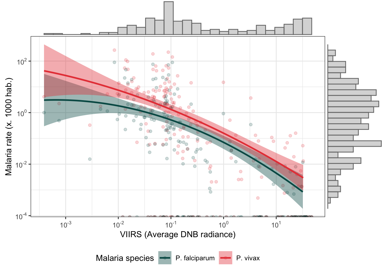
d_v_yy %>%
  mutate(r.pv = r.pv*1000,
         r.pf = r.pf*1000) %>%
  dplyr::select(r.pv, r.pf, ADM2_ES, viirs) %>%
  gather(type, rate, r.pv:r.pf) %>%
  bi_plot(trans_x = F)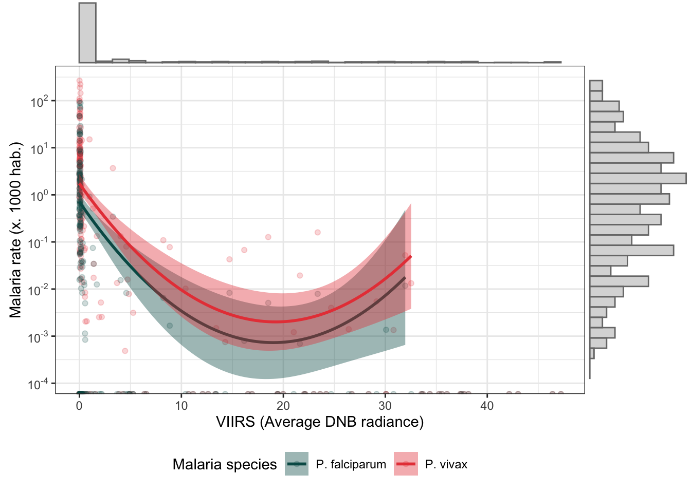
2.3 Maps
library(colorspace)
area <- st_read("./_dat/ven_admbnda_adm3_20180502/ven_admbnda_adm3_20180502.shp") %>%
  filter(ADM1_ES=="Bolivar") %>%
  mutate(ADM3_ES = toupper(ADM3_ES),
         ADM2_ES = toupper(ADM2_ES))
## Reading layer `ven_admbnda_adm3_20180502' from data source
## `/Users/gabrielcarrasco/Dropbox/Work/Colabs UCSD/NL_VEN [McCord]/Analysis/nl_ven/_dat/ven_admbnda_adm3_20180502/ven_admbnda_adm3_20180502.shp'
## using driver `ESRI Shapefile'
## Simple feature collection with 1110 features and 12 fields
## Geometry type: MULTIPOLYGON
## Dimension: XY
## Bounding box: xmin: -73.37947 ymin: 0.6345739 xmax: -59.7411 ymax: 12.19507
## Geodetic CRS: WGS 84d_v_yy <- d %>%
ungroup() %>%
group_by(Year, ADM2_ES, ADM3_ES) %>%
summarise(PV = sum(PV, na.rm = T),
PF = sum(PF, na.rm = T),
pop = sum(Population, na.rm = T),
viirs = mean(viirs, na.rm = T),
r.pv = PV/pop,
r.pf = PF/pop,
mei = mean(MEI_udel)) %>%
ungroup() %>%
mutate(cod = paste0(ADM2_ES, "-", ADM3_ES),
id = as.numeric(as.factor(cod)))
bs <- d_v_yy %>%
ungroup() %>%
group_by(ADM2_ES, ADM3_ES) %>%
summarise(viirs_init = first(viirs)+1,
viirs_last = last(viirs)+1,
pv_init = first(r.pv)+1, pv_last = last(r.pv)+1,
pf_init = first(r.pf)+1, pf_last = last(r.pf)+1,
mei_init = first(mei)+1, mei_last = last(mei)+1) %>%
ungroup() %>%
mutate(viirs_last = ifelse(viirs_last<0,0,viirs_last),
delta_viirs = 100*((viirs_last/viirs_init)-1),
delta_viirs2 = 100*((viirs_init/viirs_last)-1),
delta_pv = 100*((pv_init/pv_last)-1),
delta_pv2 = 100*((pv_last/pv_init)-1),
delta_pf = 100*((pf_init/pf_last)-1),
delta_pf2 = 100*((pf_last/pf_init)-1),
delta_mei = 100*((mei_init/mei_last)-1),
# delta_viirs = viirs_last-viirs_init,
# delta_pv = pv_last-pv_init,
# delta_pf = pf_last-pf_init,
# delta_mei = mei_last-mei_init,
cod = paste0(ADM2_ES, "-", ADM3_ES),
id = as.numeric(as.factor(cod)))
area.bs <- area %>%
inner_join(bs, by=c("ADM2_ES", "ADM3_ES")) %>%
mutate(delta_viirs_c = ntile(delta_viirs, 5),
delta_pv_c = ntile(delta_pv, 5),
delta_pf_c = ntile(delta_pf, 5),
delta_mei_c = ntile(delta_mei, 5))
# Bolivar
bs.a <- area.bs %>%
ggplot() +
geom_sf(aes(fill=delta_viirs), size = .1) +
#scale_fill_discrete_sequential("viridis") +
scale_fill_continuous_sequential(palette = "Rocket", rev = F) +
theme_bw() +
labs(fill = "viirs % variation \n(ref: 2012)") +
theme(legend.position = "bottom")
limit <- max(abs(area.bs$delta_mei)) * c(-1, 1)
bs.b <- area.bs %>%
ggplot() +
geom_sf(aes(fill=delta_mei), size = .1) +
# scale_fill_discrete_sequential("viridis") +
scale_fill_continuous_diverging(palette = "Blue-Red 3",
limit = limit) +
theme_bw() +
labs(fill = "MEI % variation \n(ref: 2016)") +
theme(legend.position = "bottom")
limit <- max(abs(area.bs$delta_pv)) * c(-1, 1)
bs.c <- area.bs %>%
ggplot() +
geom_sf(aes(fill=delta_pv), size = .1) +
# scale_fill_discrete_sequential("RedOr") +
scale_fill_continuous_diverging(palette = "Vik",
limit = limit) +
theme_bw() +
labs(fill = "Pv % variation \n(ref: 2016)") +
theme(legend.position = "bottom")
limit <- max(abs(area.bs$delta_pf)) * c(-1, 1)
bs.d <- area.bs %>%
ggplot() +
geom_sf(aes(fill=delta_pf), size = .1) +
# scale_fill_discrete_sequential("RedOr") +
scale_fill_continuous_diverging(palette = "Vik",
limit = limit) +
theme_bw() +
labs(fill = "Pf % variation \n(ref: 2016)") +
theme(legend.position = "bottom")
library(cowplot)
plot_grid(bs.a, bs.b, bs.c, bs.d, nrow = 2)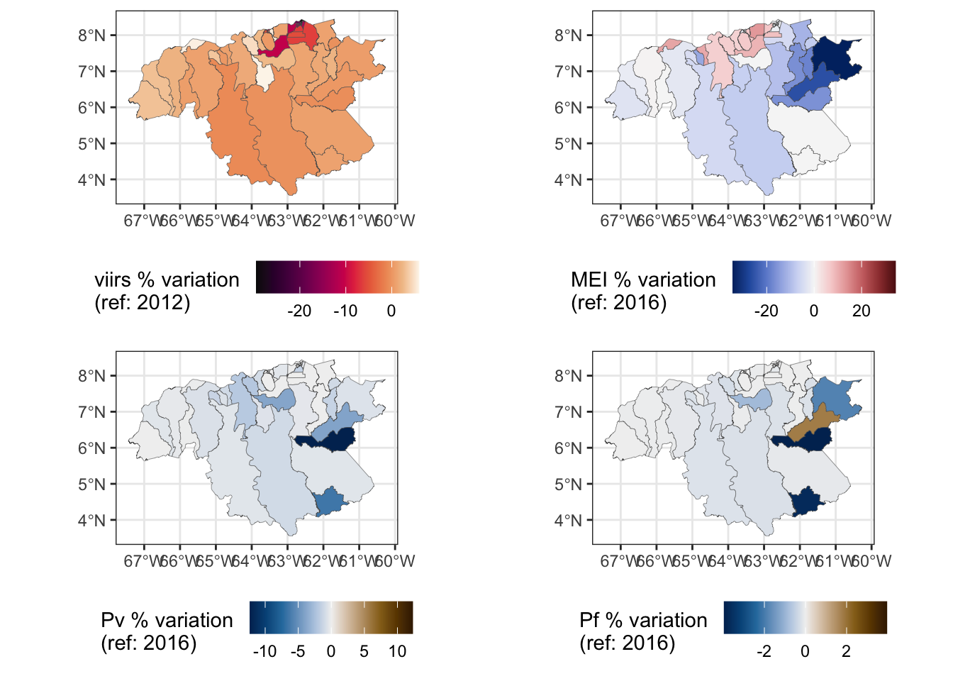
2.4 Figure 1
f1a <- d_v_yy %>%
  mutate(r.pv = r.pv*1000,
         r.pf = r.pf*1000) %>%
  dplyr::select(r.pv, r.pf, ADM2_ES, viirs) %>%
  gather(type, rate, r.pv:r.pf) %>%
  bi_plot()

#devtools::install_github("kwstat/pals")
library(pals)

limit <- c(-15, 15)

range(area.bs$delta_viirs)
## [1] -29.492028 5.940765range(area.bs$delta_pv2)## [1] -0.0200908 14.0391706range(area.bs$delta_pf2)## [1] -1.777795 4.125185aa <- area.bs %>%
mutate(x = 1) %>%
group_by(x) %>%
summarise(x = mean(x))
bb <- area.bs %>%
select(delta_viirs, delta_pv2, delta_pf2) %>%
gather(key = var, value = val, delta_viirs:delta_pf2) %>%
ggplot() +
geom_sf(aes(fill=val), size = .1) +
geom_sf(data = aa, fill = NA, size = .6) +
scale_fill_gradientn(colours=ocean.curl(100), guide = "colourbar",
limit = limit) +
theme_void() +
facet_wrap(.~var, nrow = 1,
labeller = as_labeller(c(`delta_pf2` = "P. falciparum",
`delta_pv2` = "P. vivax",
`delta_viirs` = "VIIRS"))
) +
labs(fill = "% variation \n(ref: 2012)") +
theme(legend.position = "bottom")
library(cowplot)
f1 <- plot_grid(f1a, bb, ncol = 1, labels = c("A)", "B)"))
f1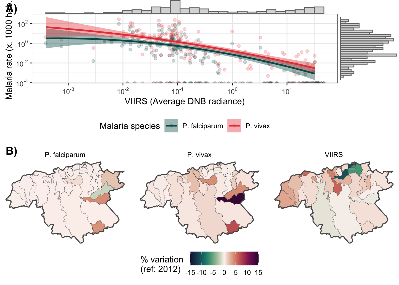
ggsave(plot =  f1, filename = "./_out/fig1.png", width = 7, height = 6,
       dpi = "retina", bg = "white")