Chapter 3 Model Falciparum
3.1 Packages and functions
rm(list=ls())
library(tidyverse)
library(purrr)
load("./_dat/NL_VEN_dat.RData")

# Bayes

library(INLA)
library(spdep)
library(purrr)
devtools::source_gist("https://gist.github.com/gcarrascoe/89e018d99bad7d3365ec4ac18e3817bd")

inla.batch <- function(formula, dat1 = dt_final) {
  result = inla(formula, data=dat1, family="nbinomial",
                offset=log(pop), verbose = F,
                #control.inla=list(strategy="gaussian"),
                control.compute=list(config=T, dic=T, cpo=T, waic=T),
                control.fixed = list(correlation.matrix=T),
                control.predictor=list(link=1,compute=TRUE)
                )
  return(result)
}

inla.batch.safe <- possibly(inla.batch, otherwise = NA_real_)

inla.batch2 <- function(formula, dat1 = dt_final) {
  result = inla(formula, data=dat1, family="gaussian",
                verbose = F,
                #control.inla=list(strategy="gaussian"),
                control.compute=list(config=T, dic=T, cpo=T, waic=T),
                control.fixed = list(correlation.matrix=T),
                control.predictor=list(link=1,compute=TRUE)
                )
  return(result)
}

inla.batch.safe2 <- possibly(inla.batch2, otherwise = NA_real_)
3.2 Mean Model
3.2.1 M: Data
#Create adjacency matrix
n <- nrow(dt_final)
nb.map <- poly2nb(area.bs)
nb2INLA("./map.graph",nb.map)

codes<-as.data.frame(area.bs)
codes$index<-as.numeric(row.names(codes))
codes<-subset(codes,select=c("cod","index"))

dt_final <- d_v_yy %>%
  filter(Year > 2013) %>%
  merge(codes, by="cod") %>%
  mutate(r.pf = r.pf*100000,
         r.pv = r.pv*100000, # Malaria rate / API * 100,000 hab
         viirs = viirs/10) #%>% # VIIRS Scales (per 10 units)
  # group_by(index) %>%
  # mutate(mei = scale_this(mei),
  #        tmmx = scale_this(tmmx),
  #        pr = scale_this(pr))
3.2.2 M: OLS
library(plm)
hist(dt_final$r.pf)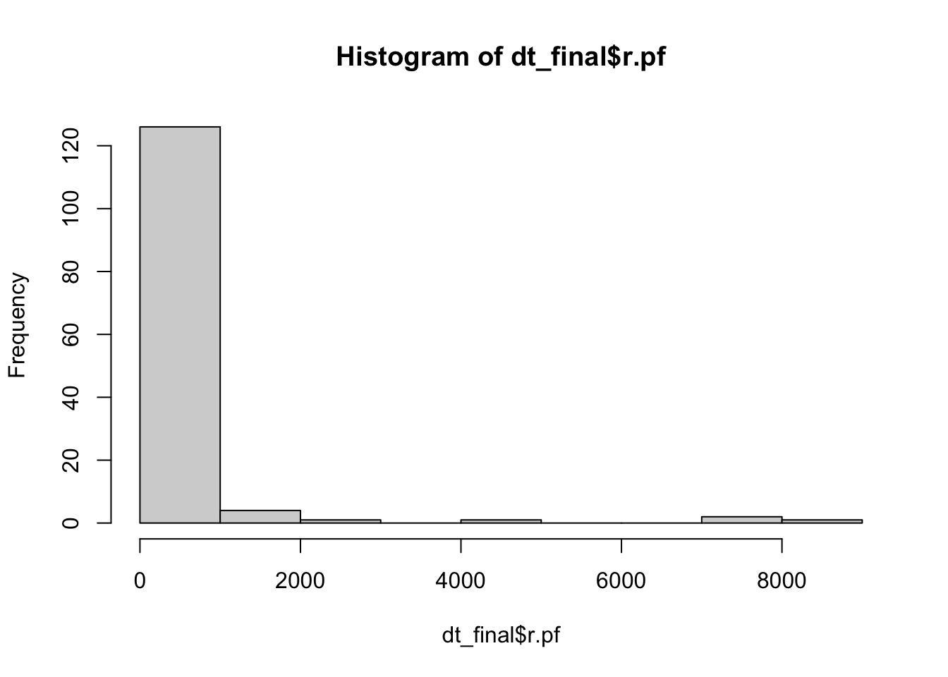
fe_1 <- plm(r.pf ~ viirs + tmmx + pr,
            data = dt_final,
            index = c("index", "Year"),
            model = "within")

summary(fe_1)
## Oneway (individual) effect Within Model
##
## Call:
## plm(formula = r.pf ~ viirs + tmmx + pr, data = dt_final, model = "within",
## index = c("index", "Year"))
##
## Balanced Panel: n = 45, T = 3, N = 135
##
## Residuals:
## Min. 1st Qu. Median 3rd Qu. Max.
## -1320.6901 -33.6956 -7.9843 37.5520 1931.3933
##
## Coefficients:
## Estimate Std. Error t-value Pr(>|t|)
## viirs 8.5490e+01 2.0485e+02 0.4173 0.6775
## tmmx 1.7553e+02 1.7289e+02 1.0153 0.3128
## pr 4.3192e-06 5.0085e-06 0.8624 0.3909
##
## Total Sum of Squares: 12347000
## Residual Sum of Squares: 11967000
## R-Squared: 0.030734
## Adj. R-Squared: -0.49289
## F-statistic: 0.919544 on 3 and 87 DF, p-value: 0.43494re_1 <- plm(r.pf ~ viirs + tmmx + pr,
data = dt_final,
index = c("index", "Year"),
model = "random")
summary(re_1)## Oneway (individual) effect Random Effect Model
## (Swamy-Arora's transformation)
##
## Call:
## plm(formula = r.pf ~ viirs + tmmx + pr, data = dt_final, model = "random",
## index = c("index", "Year"))
##
## Balanced Panel: n = 45, T = 3, N = 135
##
## Effects:
## var std.dev share
## idiosyncratic 137554.9 370.9 0.091
## individual 1381404.7 1175.3 0.909
## theta: 0.8208
##
## Residuals:
## Min. 1st Qu. Median 3rd Qu. Max.
## -950.175 -80.347 -43.878 -18.624 2381.150
##
## Coefficients:
## Estimate Std. Error z-value Pr(>|z|)
## (Intercept) 3.2649e+03 4.2536e+03 0.7676 0.4427
## viirs -8.6456e+01 1.2463e+02 -0.6937 0.4879
## tmmx -7.6874e+01 1.1164e+02 -0.6886 0.4911
## pr 5.2469e-06 4.1184e-06 1.2740 0.2027
##
## Total Sum of Squares: 18855000
## Residual Sum of Squares: 18483000
## R-Squared: 0.019745
## Adj. R-Squared: -0.0027037
## Chisq: 2.63868 on 3 DF, p-value: 0.450753.2.3 M: Clustered
library(estimatr)

mod <- lm_robust(r.pf ~ viirs + tmmx + pr, data = dt_final,
                clusters = ADM2_ES, fixed_effects = index)
summary(mod)
##
## Call:
## lm_robust(formula = r.pf ~ viirs + tmmx + pr, data = dt_final,
## clusters = ADM2_ES, fixed_effects = index)
##
## Standard error type: CR2
##
## Coefficients:
## Estimate Std. Error t value Pr(>|t|) CI Lower CI Upper DF
## viirs 8.549e+01 9.115e+01 0.9379 0.4823 -5.296e+02 7.006e+02 1.388
## tmmx 1.755e+02 1.524e+02 1.1520 0.2842 -1.790e+02 5.300e+02 7.615
## pr 4.319e-06 3.603e-06 1.1987 0.3419 -9.681e-06 1.832e-05 2.243
##
## Multiple R-squared: 0.9443 , Adjusted R-squared: 0.9142
## Multiple R-squared (proj. model): 0.03073 , Adjusted R-squared (proj. model): -0.4929
## F-statistic (proj. model): 0.7434 on 3 and 10 DF, p-value: 0.5503mod2 <- lm_robust(r.pf ~ viirs + tmmx + pr + as.factor(Year) + ADM3_ES,
data = dt_final, clusters = ADM2_ES, se_type = "stata")
#summary(mod2)
tidy(mod2) %>%
filter(term %in% c("viirs", "tmmx", "pr"))## term estimate std.error statistic p.value conf.low
## 1 viirs -2.870460e+02 1.190765e+02 -2.410601 0.03664571 -5.523650e+02
## 2 tmmx -4.470629e+02 3.029699e+02 -1.475602 0.17082916 -1.122122e+03
## 3 pr 5.815275e-06 5.754278e-06 1.010600 0.33603517 -7.006055e-06
## conf.high df outcome
## 1 -2.172695e+01 10 r.pf
## 2 2.279961e+02 10 r.pf
## 3 1.863661e-05 10 r.pf3.2.4 M: Zero Inflated
library(glmmTMB)
hist(dt_final$PF)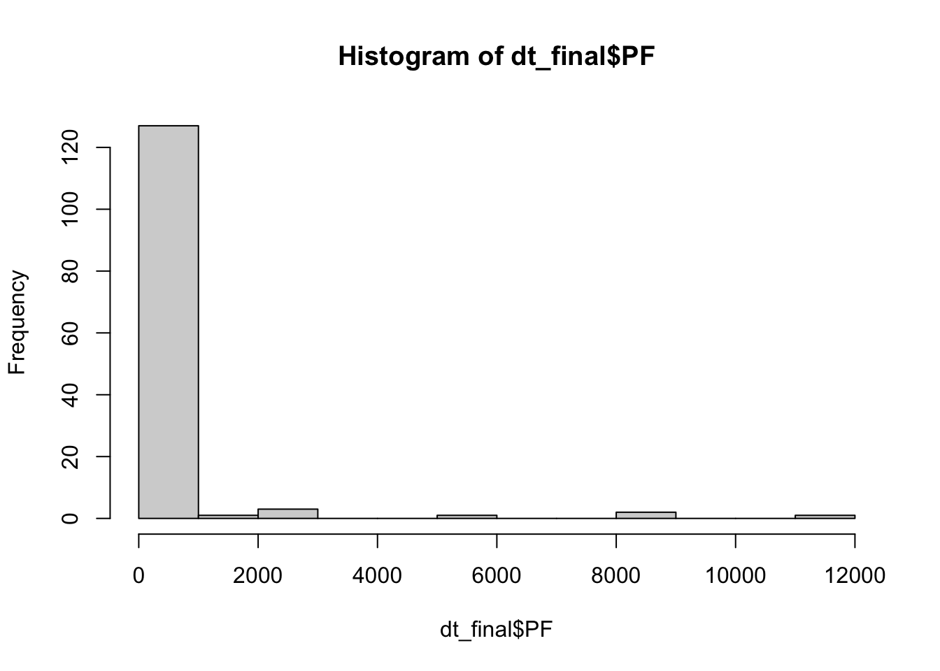
zi_1 <- glmmTMB(PF ~ viirs + tmmx + pr + (1|index) + (1|Year) +
                  offset(log(pop)), data = dt_final,
                ziformula=~1, family="nbinom2")

summary(zi_1)
## Family: nbinom2 ( log )
## Formula:
## PF ~ viirs + tmmx + pr + (1 | index) + (1 | Year) + offset(log(pop))
## Zero inflation: ~1
## Data: dt_final
##
## AIC BIC logLik deviance df.resid
## NA NA NA NA 127
##
## Random effects:
##
## Conditional model:
## Groups Name Variance Std.Dev.
## index (Intercept) 11.586 3.404
## Year (Intercept) 1.359 1.166
## Number of obs: 135, groups: index, 45; Year, 3
##
## Overdispersion parameter for nbinom2 family (): 1.03
##
## Conditional model:
## Estimate Std. Error z value Pr(>|z|)
## (Intercept) 1.307e+01 NaN NaN NaN
## viirs -3.324e+00 NaN NaN NaN
## tmmx -5.618e-01 NaN NaN NaN
## pr -1.681e-08 NaN NaN NaN
##
## Zero-inflation model:
## Estimate Std. Error z value Pr(>|z|)
## (Intercept) -25.23 NaN NaN NaN3.2.5 M: Bayesian Spatio-temporal
# MODEL
pf_2<-c(formula = PF ~ 1,
        formula = PF ~ 1 + viirs + tmmx + pr +
          f(index, model = "bym", graph = "./map.graph") +
          f(Year, model = "iid"))

# ------------------------------------------
# PF estimation
# ------------------------------------------
names(pf_2)<-pf_2

test_pf_2 <- pf_2 %>% purrr::map(~inla.batch.safe(formula = .))

(pf_2.s <- test_pf_2 %>%
  purrr::map(~Rsq.batch.safe(model = ., n = n,
                             dic.null = test_pf_2[[1]]$dic)) %>%
  bind_rows(.id = "formula") %>% mutate(id = row_number()))
## [1] 0
## [1] 0.2701045## # A tibble: 2 × 8
## formula Rsq DIC pD `log score` waic `waic pD` id
## <chr> <dbl> <dbl> <dbl> <dbl> <dbl> <dbl> <int>
## 1 "PF ~ 1" 0 1303. 1.85 4.83 1304. 2.70 1
## 2 "PF ~ 1 + viirs + tmmx + … 0.270 1238. 5.02 5.59 1241. 6.55 2pf_2.s %>%
plot_score()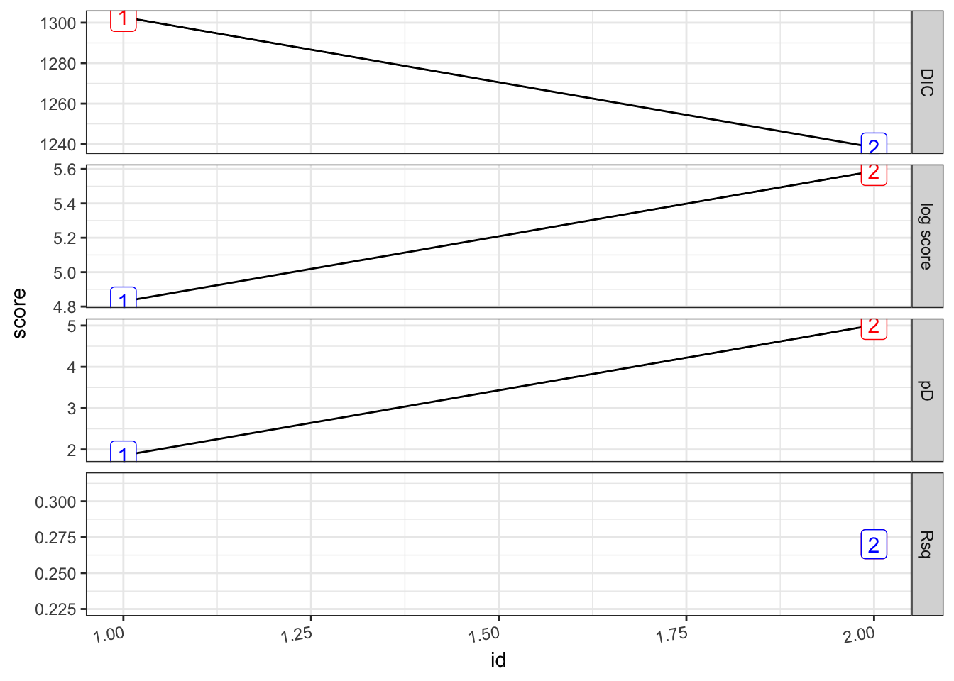
# Sumamry
summary(test_pf_2[[2]])
##
## Call:
## c("inla(formula = formula, family = \"nbinomial\", data = dat1, offset
## = log(pop), ", " verbose = F, control.compute = list(config = T, dic =
## T, ", " cpo = T, waic = T), control.predictor = list(link = 1, ", "
## compute = TRUE), control.fixed = list(correlation.matrix = T))" )
## Time used:
## Pre = 5.01, Running = 1.21, Post = 0.203, Total = 6.42
## Fixed effects:
## mean sd 0.025quant 0.5quant 0.975quant mode kld
## (Intercept) 36.863 8.176 21.032 36.783 53.148 36.628 0
## viirs -2.153 0.204 -2.541 -2.157 -1.738 -2.165 0
## tmmx -1.139 0.215 -1.565 -1.137 -0.721 -1.135 0
## pr 0.000 0.000 0.000 0.000 0.000 0.000 0
##
## Linear combinations (derived):
## ID mean sd 0.025quant 0.5quant 0.975quant mode kld
## (Intercept) 1 36.865 8.175 20.771 36.873 52.898 36.890 0
## viirs 2 -2.153 0.204 -2.554 -2.153 -1.751 -2.153 0
## tmmx 3 -1.139 0.215 -1.560 -1.139 -0.717 -1.140 0
## pr 4 0.000 0.000 0.000 0.000 0.000 0.000 0
##
## Random effects:
## Name Model
## index BYM model
## Year IID model
##
## Model hyperparameters:
## mean sd
## size for the nbinomial observations (1/overdispersion) 1.94e-01 2.20e-02
## Precision for index (iid component) 1.48e+03 1.36e+03
## Precision for index (spatial component) 2.39e+03 2.53e+03
## Precision for Year 2.10e+04 2.01e+04
## 0.025quant 0.5quant
## size for the nbinomial observations (1/overdispersion) 0.154 1.92e-01
## Precision for index (iid component) 92.718 1.09e+03
## Precision for index (spatial component) 225.892 1.64e+03
## Precision for Year 2326.945 1.52e+04
## 0.975quant mode
## size for the nbinomial observations (1/overdispersion) 2.39e-01 0.191
## Precision for index (iid component) 5.07e+03 251.302
## Precision for index (spatial component) 9.12e+03 622.294
## Precision for Year 7.39e+04 6512.616
##
## Expected number of effective parameters(stdev): 4.03(0.037)
## Number of equivalent replicates : 33.50
##
## Deviance Information Criterion (DIC) ...............: 1238.33
## Deviance Information Criterion (DIC, saturated) ....: -159.84
## Effective number of parameters .....................: 5.01
##
## Watanabe-Akaike information criterion (WAIC) ...: 1241.42
## Effective number of parameters .................: 6.55
##
## Marginal log-Likelihood: -652.13
## CPO and PIT are computed
##
## Posterior marginals for the linear predictor and
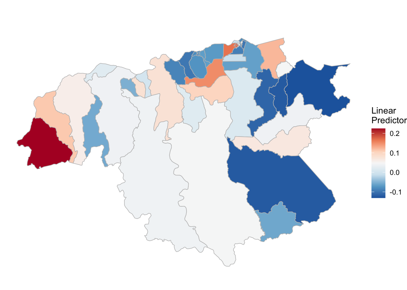
## the fitted values are computed(rm_pf_1 <- test_pf_2[[2]] %>% plot_random_map2(map = area.bs, name= "", id = cod, col1 = "gray"))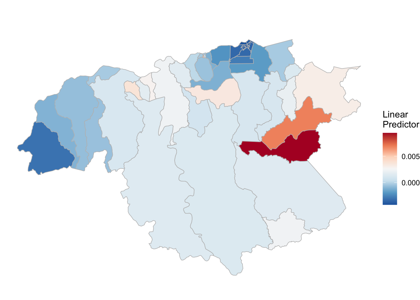
3.3 Variation model (Ref start)
3.3.1 VS: Data
dt_final_rs <- dt_final %>%
  arrange(ADM2_ES, ADM3_ES, cod, Year) %>%
  group_by(cod) %>%
  mutate(PV = PV + 1,
         PF = PF + 1,
         r.pv = PV/pop,
         r.pf = PF/pop) %>%
  mutate_at(.vars = c("r.pv", "r.pf", "viirs", "PV", "PF"),
            ~((./first(.))-1)) %>%
  filter(Year > 2013)
3.3.2 VS: OLS
library(plm)
hist(dt_final_rs$PF)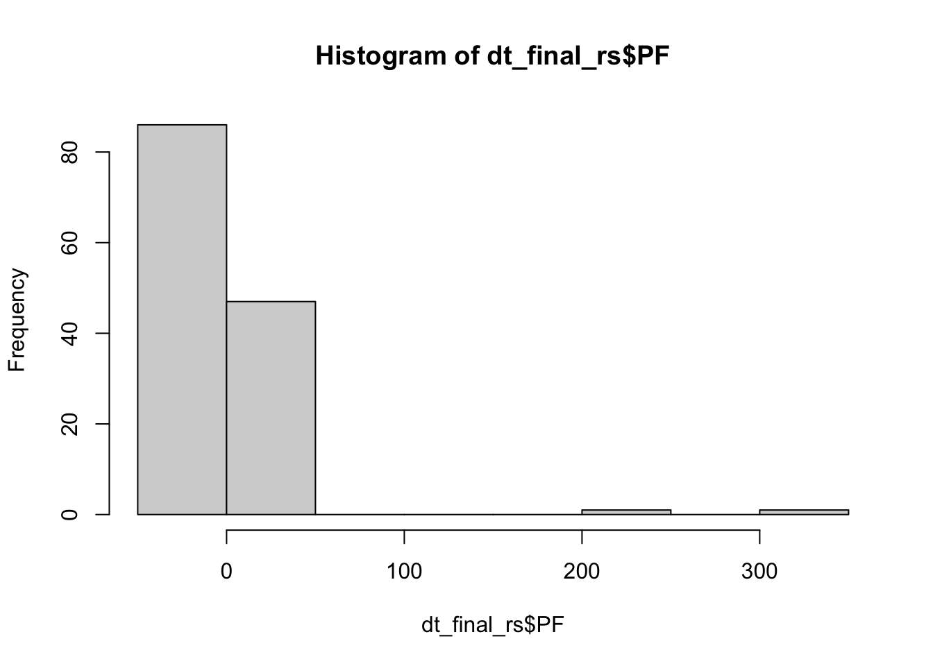
fe_1 <- plm(PF ~ viirs + tmmx + pr,
            data = dt_final_rs,
            index = c("index", "Year"),
            model = "within")

summary(fe_1)
## Oneway (individual) effect Within Model
##
## Call:
## plm(formula = PF ~ viirs + tmmx + pr, data = dt_final_rs, model = "within",
## index = c("index", "Year"))
##
## Balanced Panel: n = 45, T = 3, N = 135
##
## Residuals:
## Min. 1st Qu. Median 3rd Qu. Max.
## -96.84234 -6.25413 0.18614 5.80974 192.53372
##
## Coefficients:
## Estimate Std. Error t-value Pr(>|t|)
## viirs -7.7740e+00 6.5094e+00 -1.1943 0.23562
## tmmx 2.7183e+01 1.3264e+01 2.0494 0.04344 *
## pr -1.9827e-08 4.9271e-07 -0.0402 0.96799
## ---
## Signif. codes: 0 '***' 0.001 '**' 0.01 '*' 0.05 '.' 0.1 ' ' 1
##
## Total Sum of Squares: 94611
## Residual Sum of Squares: 86914
## R-Squared: 0.081359
## Adj. R-Squared: -0.41492
## F-statistic: 2.56838 on 3 and 87 DF, p-value: 0.059524re_1 <- plm(PF ~ viirs + tmmx + pr,
data = dt_final_rs,
index = c("index", "Year"),
model = "random")
summary(re_1)## Oneway (individual) effect Random Effect Model
## (Swamy-Arora's transformation)
##
## Call:
## plm(formula = PF ~ viirs + tmmx + pr, data = dt_final_rs, model = "random",
## index = c("index", "Year"))
##
## Balanced Panel: n = 45, T = 3, N = 135
##
## Effects:
## var std.dev share
## idiosyncratic 999.007 31.607 0.998
## individual 1.816 1.348 0.002
## theta: 0.002715
##
## Residuals:
## Min. 1st Qu. Median 3rd Qu. Max.
## -17.6047 -7.1414 -5.6576 -1.3098 292.3514
##
## Coefficients:
## Estimate Std. Error z-value Pr(>|z|)
## (Intercept) 7.8269e+01 1.0677e+02 0.7331 0.46351
## viirs -9.4120e+00 5.2199e+00 -1.8031 0.07137 .
## tmmx -1.8939e+00 2.7891e+00 -0.6790 0.49711
## pr -2.1348e-08 1.3092e-07 -0.1631 0.87047
## ---
## Signif. codes: 0 '***' 0.001 '**' 0.01 '*' 0.05 '.' 0.1 ' ' 1
##
## Total Sum of Squares: 137100
## Residual Sum of Squares: 133570
## R-Squared: 0.025748
## Adj. R-Squared: 0.0034366
## Chisq: 3.46209 on 3 DF, p-value: 0.325713.3.3 VS: Clustered
library(estimatr)

mod <- lm_robust(PF ~ viirs + tmmx + pr, data = dt_final_rs,
                clusters = ADM2_ES, fixed_effects = index)
summary(mod)
##
## Call:
## lm_robust(formula = PF ~ viirs + tmmx + pr, data = dt_final_rs,
## clusters = ADM2_ES, fixed_effects = index)
##
## Standard error type: CR2
##
## Coefficients:
## Estimate Std. Error t value Pr(>|t|) CI Lower CI Upper DF
## viirs -7.774e+00 5.122e+00 -1.51782 0.1986 -2.160e+01 6.050e+00 4.312
## tmmx 2.718e+01 1.473e+01 1.84533 0.1188 -9.632e+00 6.400e+01 5.522
## pr -1.983e-08 3.633e-07 -0.05458 0.9607 -1.361e-06 1.321e-06 2.393
##
## Multiple R-squared: 0.3671 , Adjusted R-squared: 0.0252
## Multiple R-squared (proj. model): 0.08136 , Adjusted R-squared (proj. model): -0.4149
## F-statistic (proj. model): 1.288 on 3 and 10 DF, p-value: 0.3314mod2 <- lm_robust(PF ~ viirs + tmmx + pr + as.factor(Year) + ADM3_ES,
data = dt_final_rs, clusters = ADM2_ES, se_type = "stata")
#summary(mod2)
tidy(mod2) %>%
filter(term %in% c("viirs", "tmmx", "pr"))## term estimate std.error statistic p.value conf.low
## 1 viirs 2.016580e+00 6.587744e+00 0.3061108 0.7657983 -1.266183e+01
## 2 tmmx 2.229313e+01 2.330454e+01 0.9566005 0.3613232 -2.963261e+01
## 3 pr 8.167522e-08 3.976117e-07 0.2054145 0.8413695 -8.042589e-07
## conf.high df outcome
## 1 1.669499e+01 10 PF
## 2 7.421887e+01 10 PF
## 3 9.676094e-07 10 PF3.3.4 VS: Zero Inflated
library(glmmTMB)

# zi_1 <- glmmTMB(PF ~ viirs + tmmx + pr + (1|index) + (1|Year),
#                 data = dt_final_rs,
#                 ziformula=~1, family = "gaussian")

#summary(zi_1)
3.3.5 VS: Bayesian Spatio-temporal
# MODEL
pf_2<-c(formula = PF ~ 1,
        formula = PF ~ 1 + viirs + tmmx + pr +
          f(index, model = "bym", graph = "./map.graph") +
          f(Year, model = "iid"))

# ------------------------------------------
# PF estimation
# ------------------------------------------
names(pf_2)<-pf_2

test_pf_2 <- pf_2 %>%
  purrr::map(~inla.batch.safe2(formula = ., dat1 = dt_final_rs))

(pf_2.s <- test_pf_2 %>%
  purrr::map(~Rsq.batch.safe(model = ., n = n,
                             dic.null = test_pf_2[[1]]$dic)) %>%
  bind_rows(.id = "formula") %>% mutate(id = row_number()))
## [1] 0
## [1] 0.01549469## # A tibble: 2 × 8
## formula Rsq DIC pD `log score` waic `waic pD` id
## <chr> <dbl> <dbl> <dbl> <dbl> <dbl> <dbl> <int>
## 1 "PF ~ 1" 0 1322. 2.07 5.02 1371. 37.8 1
## 2 "PF ~ 1 + viirs + tmmx +… 0.0155 1324. 4.93 4.98 1366. 33.8 2pf_2.s %>%
plot_score()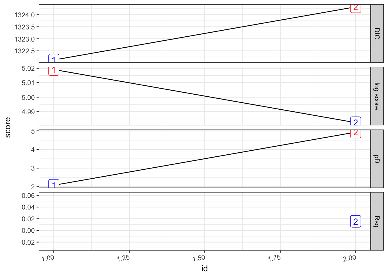
# Sumamry
summary(test_pf_2[[2]])
##
## Call:
## c("inla(formula = formula, family = \"gaussian\", data = dat1, verbose
## = F, ", " control.compute = list(config = T, dic = T, cpo = T, waic =
## T), ", " control.predictor = list(link = 1, compute = TRUE),
## control.fixed = list(correlation.matrix = T))" )
## Time used:
## Pre = 5.03, Running = 0.559, Post = 0.217, Total = 5.81
## Fixed effects:
## mean sd 0.025quant 0.5quant 0.975quant mode kld
## (Intercept) 77.151 105.865 -131.045 77.158 285.068 77.180 0
## viirs -9.159 5.138 -19.257 -9.161 0.938 -9.164 0
## tmmx -1.865 2.766 -7.302 -1.865 3.568 -1.865 0
## pr 0.000 0.000 0.000 0.000 0.000 0.000 0
##
## Linear combinations (derived):
## ID mean sd 0.025quant 0.5quant 0.975quant mode kld
## (Intercept) 1 77.151 105.865 -131.045 77.158 285.068 77.180 0
## viirs 2 -9.159 5.138 -19.257 -9.161 0.938 -9.164 0
## tmmx 3 -1.865 2.766 -7.302 -1.865 3.568 -1.865 0
## pr 4 0.000 0.000 0.000 0.000 0.000 0.000 0
##
## Random effects:
## Name Model
## index BYM model
## Year IID model
##
## Model hyperparameters:
## mean sd 0.025quant 0.5quant
## Precision for the Gaussian observations 1.00e-03 0.00 0.001 1.00e-03
## Precision for index (iid component) 2.23e+03 2197.32 254.385 1.59e+03
## Precision for index (spatial component) 3.11e+03 2326.85 758.363 2.46e+03
## Precision for Year 2.34e+04 16697.41 4375.319 1.93e+04
## 0.975quant mode
## Precision for the Gaussian observations 1.00e-03 1.00e-03
## Precision for index (iid component) 8.07e+03 7.00e+02
## Precision for index (spatial component) 9.42e+03 1.66e+03
## Precision for Year 6.88e+04 1.19e+04
##
## Expected number of effective parameters(stdev): 3.97(0.004)
## Number of equivalent replicates : 34.04
##
## Deviance Information Criterion (DIC) ...............: 1324.33
## Deviance Information Criterion (DIC, saturated) ....: 2977.98
## Effective number of parameters .....................: 4.93
##
## Watanabe-Akaike information criterion (WAIC) ...: 1366.48
## Effective number of parameters .................: 33.84
##
## Marginal log-Likelihood: -684.02
## CPO and PIT are computed
##
## Posterior marginals for the linear predictor and
## the fitted values are computed(rm_pf_1 <- test_pf_2[[2]] %>% plot_random_map2(map = area.bs, name= "", id = cod, col1 = "gray"))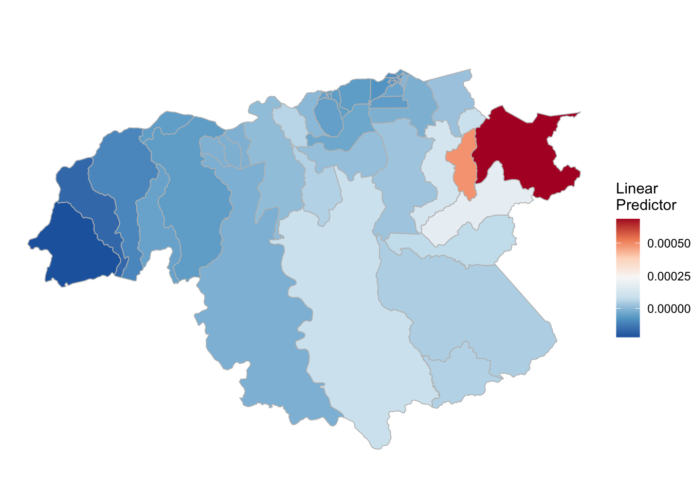
3.4 Variation model (Ref Max)
3.4.1 VM: Data
dt_final_rm <- dt_final %>%
  arrange(ADM2_ES, ADM3_ES, cod, Year) %>%
  group_by(cod) %>%
  mutate(PV = PV + 1,
         PF = PF + 1,
         r.pv = PV/pop,
         r.pf = PF/pop) %>%
  mutate_at(.vars = c("r.pv", "r.pf", "viirs", "PV", "PF"),
            ~((./max(.))-1)) %>%
  filter(Year > 2013)
3.4.2 VM: OLS
library(plm)
hist(dt_final_rm$PF)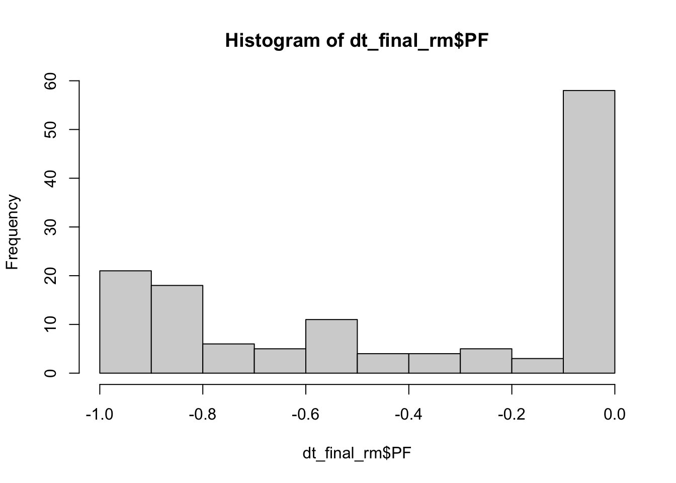
fe_1 <- plm(PF ~ viirs + tmmx + pr,
            data = dt_final_rm,
            index = c("index", "Year"),
            model = "within")

summary(fe_1)
## Oneway (individual) effect Within Model
##
## Call:
## plm(formula = PF ~ viirs + tmmx + pr, data = dt_final_rm, model = "within",
## index = c("index", "Year"))
##
## Balanced Panel: n = 45, T = 3, N = 135
##
## Residuals:
## Min. 1st Qu. Median 3rd Qu. Max.
## -0.817833 -0.201403 -0.024796 0.180881 0.527665
##
## Coefficients:
## Estimate Std. Error t-value Pr(>|t|)
## viirs -6.5188e-01 1.3607e-01 -4.7907 6.779e-06 ***
## tmmx 3.7113e-01 1.4449e-01 2.5685 0.01192 *
## pr -4.2752e-09 5.0746e-09 -0.8425 0.40184
## ---
## Signif. codes: 0 '***' 0.001 '**' 0.01 '*' 0.05 '.' 0.1 ' ' 1
##
## Total Sum of Squares: 14.874
## Residual Sum of Squares: 10.056
## R-Squared: 0.32392
## Adj. R-Squared: -0.04132
## F-statistic: 13.8943 on 3 and 87 DF, p-value: 1.7597e-07re_1 <- plm(PF ~ viirs + tmmx + pr,
data = dt_final_rm,
index = c("index", "Year"),
model = "random")
#summary(re_1)3.4.3 VM: Clustered
library(estimatr)

mod <- lm_robust(PF ~ viirs + tmmx + pr, data = dt_final_rm,
                clusters = ADM2_ES, fixed_effects = index)
summary(mod)
##
## Call:
## lm_robust(formula = PF ~ viirs + tmmx + pr, data = dt_final_rm,
## clusters = ADM2_ES, fixed_effects = index)
##
## Standard error type: CR2
##
## Coefficients:
## Estimate Std. Error t value Pr(>|t|) CI Lower CI Upper DF
## viirs -6.519e-01 2.133e-01 -3.0560 0.02571 -1.189e+00 -1.149e-01 5.375
## tmmx 3.711e-01 1.279e-01 2.9017 0.02666 5.967e-02 6.826e-01 6.121
## pr -4.275e-09 6.488e-09 -0.6589 0.56832 -2.843e-08 1.988e-08 2.367
##
## Multiple R-squared: 0.526 , Adjusted R-squared: 0.2699
## Multiple R-squared (proj. model): 0.3239 , Adjusted R-squared (proj. model): -0.04132
## F-statistic (proj. model): 7.82 on 3 and 10 DF, p-value: 0.005592mod2 <- lm_robust(PF ~ viirs + tmmx + pr + as.factor(Year) + ADM3_ES,
data = dt_final_rm, clusters = ADM2_ES, se_type = "stata")
#summary(mod2)
tidy(mod2) %>%
filter(term %in% c("viirs", "tmmx", "pr"))## term estimate std.error statistic p.value conf.low
## 1 viirs 9.657454e-04 1.263778e-01 0.007641733 0.9940531 -2.806215e-01
## 2 tmmx -3.958076e-01 2.845205e-01 -1.391138851 0.1943568 -1.029759e+00
## 3 pr -6.251712e-09 4.959618e-09 -1.260522720 0.2360986 -1.730243e-08
## conf.high df outcome
## 1 2.825530e-01 10 PF
## 2 2.381437e-01 10 PF
## 3 4.799007e-09 10 PF3.4.4 VM: Zero Inflated
library(glmmTMB)

zi_1 <- glmmTMB(PF ~ viirs + tmmx + pr + (1|index) + (1|Year),
                data = dt_final_rm,
                ziformula=~1, family=gaussian())

summary(zi_1)
## Family: gaussian ( identity )
## Formula: PF ~ viirs + tmmx + pr + (1 | index) + (1 | Year)
## Zero inflation: ~1
## Data: dt_final_rm
##
## AIC BIC logLik deviance df.resid
## 86.5 109.7 -35.2 70.5 127
##
## Random effects:
##
## Conditional model:
## Groups Name Variance Std.Dev.
## index (Intercept) 0.02264 0.1505
## Year (Intercept) 0.06495 0.2549
## Residual 0.07339 0.2709
## Number of obs: 135, groups: index, 45; Year, 3
##
## Dispersion estimate for gaussian family (sigma^2): 0.0734
##
## Conditional model:
## Estimate Std. Error z value Pr(>|z|)
## (Intercept) 1.092e+00 NaN NaN NaN
## viirs 1.676e-02 NaN NaN NaN
## tmmx -3.908e-02 NaN NaN NaN
## pr -1.281e-10 NaN NaN NaN
##
## Zero-inflation model:
## Estimate Std. Error z value Pr(>|z|)
## (Intercept) -35.93 NaN NaN NaN3.4.5 VM: Bayesian Spatio-temporal
# MODEL
pf_2<-c(formula = PF ~ 1,
        formula = PF ~ 1 + viirs + tmmx + pr +
          f(index, model = "bym", graph = "./map.graph") +
          f(Year, model = "iid"))

# ------------------------------------------
# PF estimation
# ------------------------------------------
names(pf_2)<-pf_2

test_pf_2 <- pf_2 %>%
  purrr::map(~inla.batch.safe2(formula = ., dat1 = dt_final_rm))

(pf_2.s <- test_pf_2 %>%
  purrr::map(~Rsq.batch.safe(model = ., n = n,
                             dic.null = test_pf_2[[1]]$dic)) %>%
  bind_rows(.id = "formula") %>% mutate(id = row_number()))
## [1] 0
## [1] 0.4090019## # A tibble: 2 × 8
## formula Rsq DIC pD `log score` waic `waic pD` id
## <chr> <dbl> <dbl> <dbl> <dbl> <dbl> <dbl> <int>
## 1 "PF ~ 1" 0 137. 2.07 0.506 137. 1.21 1
## 2 "PF ~ 1 + viirs + tmmx + … 0.409 65.7 25.4 0.257 67.0 23.2 2pf_2.s %>%
plot_score()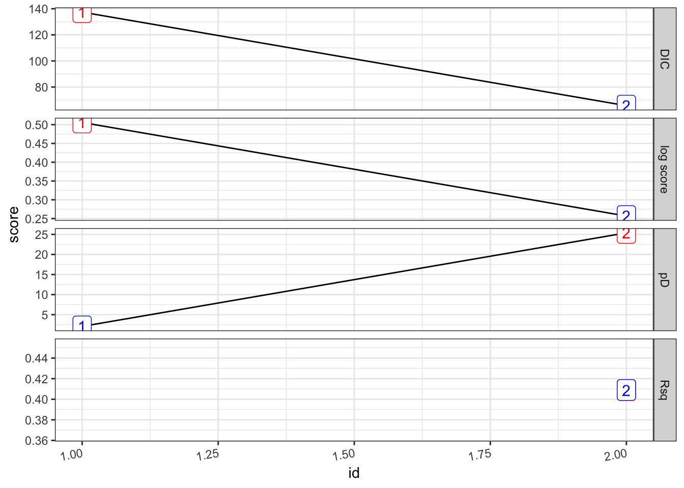
# Sumamry
summary(test_pf_2[[2]])
##
## Call:
## c("inla(formula = formula, family = \"gaussian\", data = dat1, verbose
## = F, ", " control.compute = list(config = T, dic = T, cpo = T, waic =
## T), ", " control.predictor = list(link = 1, compute = TRUE),
## control.fixed = list(correlation.matrix = T))" )
## Time used:
## Pre = 4.81, Running = 0.526, Post = 0.209, Total = 5.55
## Fixed effects:
## mean sd 0.025quant 0.5quant 0.975quant mode kld
## (Intercept) 1.037 1.290 -1.465 1.023 3.617 0.997 0
## viirs -0.001 0.137 -0.271 -0.001 0.266 0.000 0
## tmmx -0.038 0.033 -0.105 -0.037 0.027 -0.037 0
## pr 0.000 0.000 0.000 0.000 0.000 0.000 0
##
## Linear combinations (derived):
## ID mean sd 0.025quant 0.5quant 0.975quant mode kld
## (Intercept) 1 1.037 1.290 -1.465 1.023 3.617 0.997 0
## viirs 2 -0.001 0.137 -0.271 -0.001 0.266 0.000 0
## tmmx 3 -0.038 0.033 -0.105 -0.037 0.027 -0.037 0
## pr 4 0.000 0.000 0.000 0.000 0.000 0.000 0
##
## Random effects:
## Name Model
## index BYM model
## Year IID model
##
## Model hyperparameters:
## mean sd 0.025quant 0.5quant
## Precision for the Gaussian observations 13.13 2.09 9.33 13.04
## Precision for index (iid component) 114.95 125.63 25.43 76.78
## Precision for index (spatial component) 1192.44 1283.78 39.36 775.11
## Precision for Year 21.51 17.53 3.10 16.88
## 0.975quant mode
## Precision for the Gaussian observations 17.52 12.93
## Precision for index (iid component) 433.95 44.38
## Precision for index (spatial component) 4692.04 77.96
## Precision for Year 67.67 8.63
##
## Expected number of effective parameters(stdev): 22.17(7.50)
## Number of equivalent replicates : 6.09
##
## Deviance Information Criterion (DIC) ...............: 65.72
## Deviance Information Criterion (DIC, saturated) ....: -42.57
## Effective number of parameters .....................: 25.39
##
## Watanabe-Akaike information criterion (WAIC) ...: 66.96
## Effective number of parameters .................: 23.23
##
## Marginal log-Likelihood: -77.29
## CPO and PIT are computed
##
## Posterior marginals for the linear predictor and
## the fitted values are computed(rm_pf_1 <- test_pf_2[[2]] %>% plot_random_map2(map = area.bs, name= "", id = cod, col1 = "gray"))