Chapter 4 Model Vivax
4.1 Packages and functions
rm(list=ls())
library(tidyverse)
library(purrr)
load("./_dat/NL_VEN_dat.RData")

# Bayes

library(INLA)
library(spdep)
library(purrr)
devtools::source_gist("https://gist.github.com/gcarrascoe/89e018d99bad7d3365ec4ac18e3817bd")

inla.batch <- function(formula, dat1 = dt_final) {
  result = inla(formula, data=dat1, family="nbinomial",
                offset=log(pop), verbose = F,
                #control.inla=list(strategy="gaussian"),
                control.compute=list(config=T, dic=T, cpo=T, waic=T),
                control.fixed = list(correlation.matrix=T),
                control.predictor=list(link=1,compute=TRUE)
                )
  return(result)
}

inla.batch.safe <- possibly(inla.batch, otherwise = NA_real_)

inla.batch2 <- function(formula, dat1 = dt_final) {
  result = inla(formula, data=dat1, family="gaussian",
                verbose = F,
                #control.inla=list(strategy="gaussian"),
                control.compute=list(config=T, dic=T, cpo=T, waic=T),
                control.fixed = list(correlation.matrix=T),
                control.predictor=list(link=1,compute=TRUE)
                )
  return(result)
}

inla.batch.safe2 <- possibly(inla.batch2, otherwise = NA_real_)
4.2 Mean Model
4.2.1 M: Data
#Create adjacency matrix
n <- nrow(dt_final)
nb.map <- poly2nb(area.bs)
nb2INLA("./map.graph",nb.map)

codes<-as.data.frame(area.bs)
codes$index<-as.numeric(row.names(codes))
codes<-subset(codes,select=c("cod","index"))

dt_final <- d_v_yy %>%
  filter(Year > 2013) %>%
  merge(codes, by="cod") %>%
  mutate(r.pf = r.pf*100000,
         r.pv = r.pv*100000, # Malaria rate / API * 100,000 hab
         viirs = viirs/10) #%>% # VIIRS Scales (per 10 units)
  # group_by(index) %>%
  # mutate(mei = scale_this(mei),
  #        tmmx = scale_this(tmmx),
  #        pr = scale_this(pr))
4.2.2 M: OLS
library(plm)
hist(dt_final$r.pv)
fe_1 <- plm(r.pv ~ viirs + tmmx + pr,
            data = dt_final,
            index = c("index", "Year"),
            model = "within")

summary(fe_1)
## Oneway (individual) effect Within Model
##
## Call:
## plm(formula = r.pv ~ viirs + tmmx + pr, data = dt_final, model = "within",
## index = c("index", "Year"))
##
## Balanced Panel: n = 45, T = 3, N = 135
##
## Residuals:
## Min. 1st Qu. Median 3rd Qu. Max.
## -3344.301 -201.826 -46.575 159.014 3762.373
##
## Coefficients:
## Estimate Std. Error t-value Pr(>|t|)
## viirs 4.6537e+02 4.6599e+02 0.9987 0.32072
## tmmx 9.6812e+02 3.9330e+02 2.4616 0.01581 *
## pr 1.7232e-05 1.1393e-05 1.5124 0.13405
## ---
## Signif. codes: 0 '***' 0.001 '**' 0.01 '*' 0.05 '.' 0.1 ' ' 1
##
## Total Sum of Squares: 70935000
## Residual Sum of Squares: 61928000
## R-Squared: 0.12698
## Adj. R-Squared: -0.34465
## F-statistic: 4.21803 on 3 and 87 DF, p-value: 0.0078016re_1 <- plm(r.pv ~ viirs + tmmx + pr,
data = dt_final,
index = c("index", "Year"),
model = "random")
summary(re_1)## Oneway (individual) effect Random Effect Model
## (Swamy-Arora's transformation)
##
## Call:
## plm(formula = r.pv ~ viirs + tmmx + pr, data = dt_final, model = "random",
## index = c("index", "Year"))
##
## Balanced Panel: n = 45, T = 3, N = 135
##
## Effects:
## var std.dev share
## idiosyncratic 7.118e+05 8.437e+02 0.056
## individual 1.203e+07 3.468e+03 0.944
## theta: 0.8609
##
## Residuals:
## Min. 1st Qu. Median 3rd Qu. Max.
## -1280.4292 -225.8722 -145.9130 6.4648 6863.0255
##
## Coefficients:
## Estimate Std. Error z-value Pr(>|z|)
## (Intercept) -7.5822e+03 1.1017e+04 -0.6882 0.49130
## viirs -1.6431e+02 3.2868e+02 -0.4999 0.61713
## tmmx 2.2440e+02 2.8886e+02 0.7769 0.43725
## pr 2.2763e-05 1.0090e-05 2.2560 0.02407 *
## ---
## Signif. codes: 0 '***' 0.001 '**' 0.01 '*' 0.05 '.' 0.1 ' ' 1
##
## Total Sum of Squares: 104010000
## Residual Sum of Squares: 98807000
## R-Squared: 0.050037
## Adj. R-Squared: 0.028282
## Chisq: 6.90008 on 3 DF, p-value: 0.0751524.2.3 M: Clustered
library(estimatr)

mod <- lm_robust(r.pv ~ viirs + tmmx + pr, data = dt_final,
                clusters = ADM2_ES, fixed_effects = index)
summary(mod)
##
## Call:
## lm_robust(formula = r.pv ~ viirs + tmmx + pr, data = dt_final,
## clusters = ADM2_ES, fixed_effects = index)
##
## Standard error type: CR2
##
## Coefficients:
## Estimate Std. Error t value Pr(>|t|) CI Lower CI Upper DF
## viirs 4.654e+02 3.659e+02 1.272 0.37596 -2.004e+03 2.935e+03 1.388
## tmmx 9.681e+02 4.792e+02 2.020 0.07981 -1.467e+02 2.083e+03 7.615
## pr 1.723e-05 1.566e-05 1.101 0.37508 -4.360e-05 7.807e-05 2.243
##
## Multiple R-squared: 0.9652 , Adjusted R-squared: 0.9464
## Multiple R-squared (proj. model): 0.127 , Adjusted R-squared (proj. model): -0.3447
## F-statistic (proj. model): 1.791 on 3 and 10 DF, p-value: 0.2124mod2 <- lm_robust(r.pv ~ viirs + tmmx + pr + as.factor(Year) + ADM3_ES,
data = dt_final, clusters = ADM2_ES, se_type = "stata")
#summary(mod2)
tidy(mod2) %>%
filter(term %in% c("viirs", "tmmx", "pr"))## term estimate std.error statistic p.value conf.low
## 1 viirs -1.131062e+03 3.295239e+02 -3.4324125 0.006412485 -1.865287e+03
## 2 tmmx -3.142184e+03 1.482450e+03 -2.1195881 0.060065226 -6.445289e+03
## 3 pr 2.473398e-05 2.487075e-05 0.9945009 0.343433687 -3.068150e-05
## conf.high df outcome
## 1 -3.968369e+02 10 r.pv
## 2 1.609211e+02 10 r.pv
## 3 8.014947e-05 10 r.pv4.2.4 M: Zero Inflated
library(glmmTMB)
hist(dt_final$PV)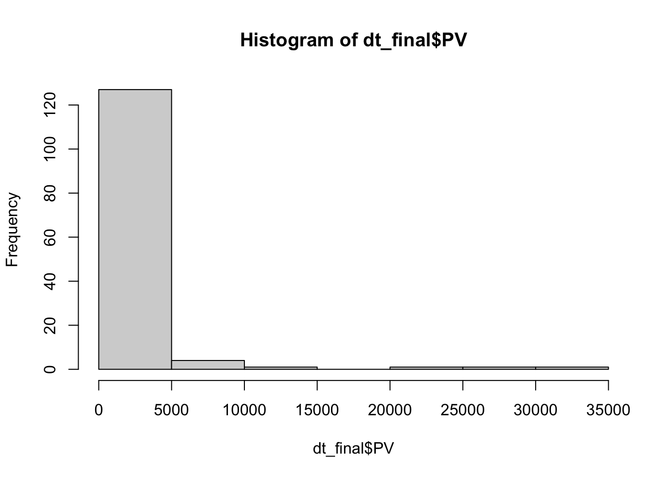
zi_1 <- glmmTMB(PV ~ viirs + tmmx + pr + (1|index) + (1|Year) +
                  offset(log(pop)), data = dt_final,
                ziformula=~1, family="nbinom2")

summary(zi_1)
## Family: nbinom2 ( log )
## Formula:
## PV ~ viirs + tmmx + pr + (1 | index) + (1 | Year) + offset(log(pop))
## Zero inflation: ~1
## Data: dt_final
##
## AIC BIC logLik deviance df.resid
## NA NA NA NA 127
##
## Random effects:
##
## Conditional model:
## Groups Name Variance Std.Dev.
## index (Intercept) 9.478 3.079
## Year (Intercept) 2.032 1.426
## Number of obs: 135, groups: index, 45; Year, 3
##
## Overdispersion parameter for nbinom2 family (): 1.39
##
## Conditional model:
## Estimate Std. Error z value Pr(>|z|)
## (Intercept) 1.694e+01 NaN NaN NaN
## viirs -2.766e+00 NaN NaN NaN
## tmmx -6.140e-01 NaN NaN NaN
## pr -3.106e-08 NaN NaN NaN
##
## Zero-inflation model:
## Estimate Std. Error z value Pr(>|z|)
## (Intercept) -3.823 NaN NaN NaN4.2.5 M: Bayesian Spatio-temporal
# MODEL
pv_2<-c(formula = PV ~ 1,
        formula = PV ~ 1 + viirs + tmmx + pr +
          f(index, model = "bym", graph = "./map.graph") +
          f(Year, model = "iid"))

# ------------------------------------------
# PV estimation
# ------------------------------------------
names(pv_2)<-pv_2

test_pv_2 <- pv_2 %>% purrr::map(~inla.batch.safe(formula = .))

(pv_2.s <- test_pv_2 %>%
  purrr::map(~Rsq.batch.safe(model = ., n = n,
                             dic.null = test_pv_2[[1]]$dic)) %>%
  bind_rows(.id = "formula") %>% mutate(id = row_number()))
## [1] 0
## [1] 0.3303684## # A tibble: 2 × 8
## formula Rsq DIC pD `log score` waic `waic pD` id
## <chr> <dbl> <dbl> <dbl> <dbl> <dbl> <dbl> <int>
## 1 "PV ~ 1" 0 1732. 1.91 6.42 1733. 2.70 1
## 2 "PV ~ 1 + viirs + tmmx + … 0.330 1652. 7.04 10.2 1652. 6.78 2pv_2.s %>%
plot_score()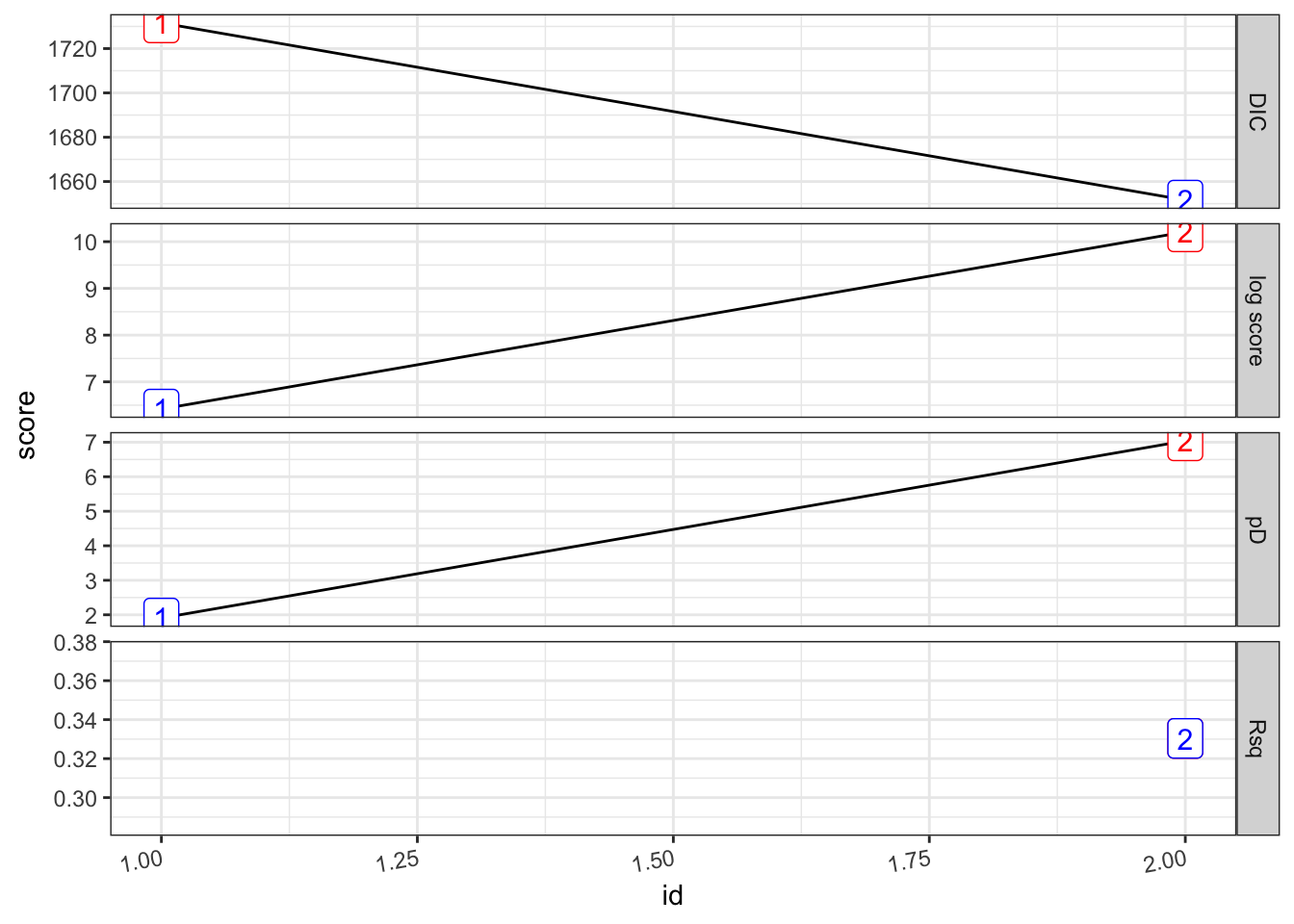
# Sumamry
summary(test_pv_2[[2]])
##
## Call:
## c("inla(formula = formula, family = \"nbinomial\", data = dat1, offset
## = log(pop), ", " verbose = F, control.compute = list(config = T, dic =
## T, ", " cpo = T, waic = T), control.predictor = list(link = 1, ", "
## compute = TRUE), control.fixed = list(correlation.matrix = T))" )
## Time used:
## Pre = 5.05, Running = 1.12, Post = 0.212, Total = 6.38
## Fixed effects:
## mean sd 0.025quant 0.5quant 0.975quant mode kld
## (Intercept) 34.906 8.134 19.158 34.830 51.108 34.690 0
## viirs -2.267 0.184 -2.620 -2.270 -1.896 -2.275 0
## tmmx -1.048 0.213 -1.472 -1.047 -0.633 -1.045 0
## pr 0.000 0.000 0.000 0.000 0.000 0.000 0
##
## Linear combinations (derived):
## ID mean sd 0.025quant 0.5quant 0.975quant mode kld
## (Intercept) 1 34.905 8.135 18.891 34.918 50.833 34.953 0
## viirs 2 -2.267 0.184 -2.630 -2.266 -1.906 -2.265 0
## tmmx 3 -1.048 0.213 -1.466 -1.049 -0.628 -1.050 0
## pr 4 0.000 0.000 0.000 0.000 0.000 0.000 0
##
## Random effects:
## Name Model
## index BYM model
## Year IID model
##
## Model hyperparameters:
## mean sd
## size for the nbinomial observations (1/overdispersion) 0.251 0.026
## Precision for index (iid component) 1817.984 1804.510
## Precision for index (spatial component) 1867.706 1876.526
## Precision for Year 4.002 5.711
## 0.025quant 0.5quant
## size for the nbinomial observations (1/overdispersion) 0.204 0.25
## Precision for index (iid component) 112.637 1280.29
## Precision for index (spatial component) 127.677 1311.15
## Precision for Year 0.314 2.30
## 0.975quant mode
## size for the nbinomial observations (1/overdispersion) 0.305 0.248
## Precision for index (iid component) 6637.643 300.795
## Precision for index (spatial component) 6818.861 348.164
## Precision for Year 18.153 0.813
##
## Expected number of effective parameters(stdev): 5.56(0.367)
## Number of equivalent replicates : 24.29
##
## Deviance Information Criterion (DIC) ...............: 1651.62
## Deviance Information Criterion (DIC, saturated) ....: -397.58
## Effective number of parameters .....................: 7.04
##
## Watanabe-Akaike information criterion (WAIC) ...: 1652.46
## Effective number of parameters .................: 6.78
##
## Marginal log-Likelihood: -866.53
## CPO and PIT are computed
##
## Posterior marginals for the linear predictor and
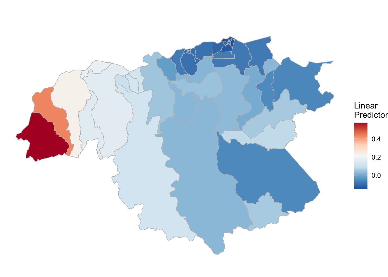
## the fitted values are computed(rm_pv_1 <- test_pv_2[[2]] %>% plot_random_map2(map = area.bs, name= "", id = cod, col1 = "gray"))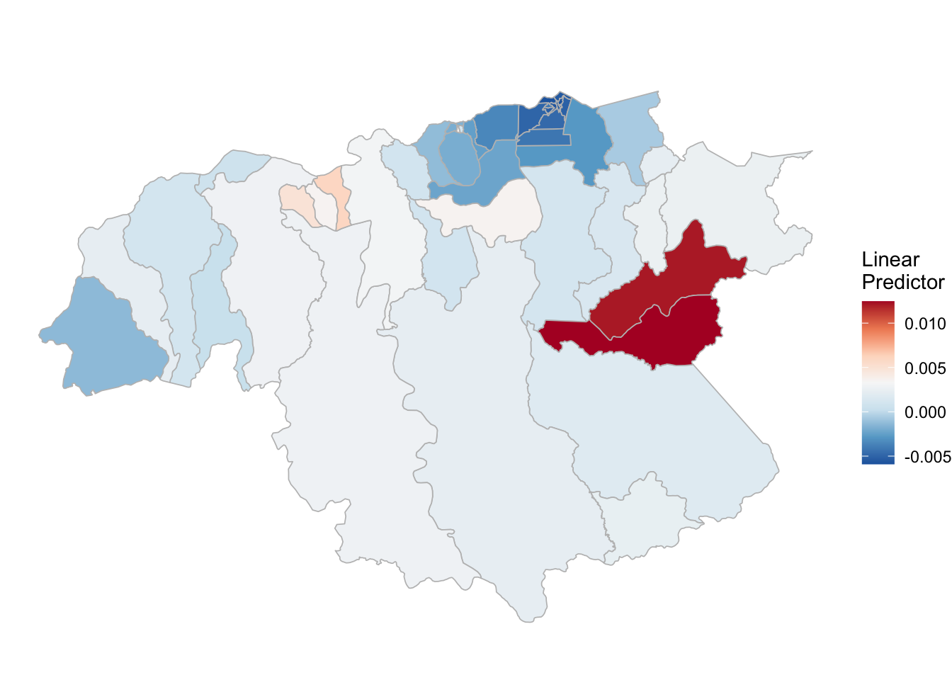
4.3 Variation model (Ref start)
4.3.1 VS: Data
dt_final_rs <- dt_final %>%
  arrange(ADM2_ES, ADM3_ES, cod, Year) %>%
  group_by(cod) %>%
  mutate(PV = PV + 1,
         PF = PF + 1,
         r.pv = PV/pop,
         r.pf = PF/pop) %>%
  mutate_at(.vars = c("r.pv", "r.pf", "viirs", "PV", "PF"),
            ~((./first(.))-1)) %>%
  filter(Year > 2013)
4.3.2 VS: OLS
library(plm)
hist(dt_final_rs$PV)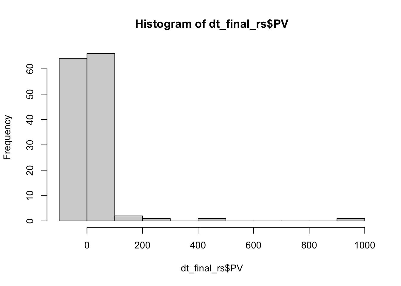
fe_1 <- plm(PV ~ viirs + tmmx + pr,
            data = dt_final_rs,
            index = c("index", "Year"),
            model = "within")

summary(fe_1)
## Oneway (individual) effect Within Model
##
## Call:
## plm(formula = PV ~ viirs + tmmx + pr, data = dt_final_rs, model = "within",
## index = c("index", "Year"))
##
## Balanced Panel: n = 45, T = 3, N = 135
##
## Residuals:
## Min. 1st Qu. Median 3rd Qu. Max.
## -295.2179 -19.7925 -4.9501 20.3364 567.3183
##
## Coefficients:
## Estimate Std. Error t-value Pr(>|t|)
## viirs -1.3789e+01 1.8136e+01 -0.7603 0.449130
## tmmx 1.1117e+02 3.6954e+01 3.0083 0.003436 **
## pr -1.1006e-06 1.3728e-06 -0.8018 0.424864
## ---
## Signif. codes: 0 '***' 0.001 '**' 0.01 '*' 0.05 '.' 0.1 ' ' 1
##
## Total Sum of Squares: 751850
## Residual Sum of Squares: 674650
## R-Squared: 0.10268
## Adj. R-Squared: -0.38208
## F-statistic: 3.31854 on 3 and 87 DF, p-value: 0.023551re_1 <- plm(PV ~ viirs + tmmx + pr,
data = dt_final_rs,
index = c("index", "Year"),
model = "random")
summary(re_1)## Oneway (individual) effect Random Effect Model
## (Swamy-Arora's transformation)
##
## Call:
## plm(formula = PV ~ viirs + tmmx + pr, data = dt_final_rs, model = "random",
## index = c("index", "Year"))
##
## Balanced Panel: n = 45, T = 3, N = 135
##
## Effects:
## var std.dev share
## idiosyncratic 7754.62 88.06 0.984
## individual 122.34 11.06 0.016
## theta: 0.02286
##
## Residuals:
## Min. 1st Qu. Median 3rd Qu. Max.
## -39.3814 -23.8523 -21.7070 -4.7319 885.3256
##
## Coefficients:
## Estimate Std. Error z-value Pr(>|z|)
## (Intercept) 5.2628e+01 3.0781e+02 0.1710 0.8642
## viirs -1.8203e+01 1.4819e+01 -1.2284 0.2193
## tmmx -7.5006e-01 8.0412e+00 -0.0933 0.9257
## pr -3.1535e-07 3.7727e-07 -0.8359 0.4032
##
## Total Sum of Squares: 1086600
## Residual Sum of Squares: 1069200
## R-Squared: 0.016
## Adj. R-Squared: -0.0065348
## Chisq: 2.13002 on 3 DF, p-value: 0.545864.3.3 VS: Clustered
library(estimatr)

mod <- lm_robust(PV ~ viirs + tmmx + pr, data = dt_final_rs,
                clusters = ADM2_ES, fixed_effects = index)
summary(mod)
##
## Call:
## lm_robust(formula = PV ~ viirs + tmmx + pr, data = dt_final_rs,
## clusters = ADM2_ES, fixed_effects = index)
##
## Standard error type: CR2
##
## Coefficients:
## Estimate Std. Error t value Pr(>|t|) CI Lower CI Upper DF
## viirs -1.379e+01 1.009e+01 -1.367 0.2387 -4.102e+01 1.344e+01 4.312
## tmmx 1.112e+02 5.685e+01 1.955 0.1025 -3.092e+01 2.533e+02 5.522
## pr -1.101e-06 6.600e-07 -1.668 0.2165 -3.537e-06 1.336e-06 2.393
##
## Multiple R-squared: 0.388 , Adjusted R-squared: 0.05744
## Multiple R-squared (proj. model): 0.1027 , Adjusted R-squared (proj. model): -0.3821
## F-statistic (proj. model): 1.522 on 3 and 10 DF, p-value: 0.2686mod2 <- lm_robust(PV ~ viirs + tmmx + pr + as.factor(Year) + ADM3_ES,
data = dt_final_rs, clusters = ADM2_ES, se_type = "stata")
#summary(mod2)
tidy(mod2) %>%
filter(term %in% c("viirs", "tmmx", "pr"))## term estimate std.error statistic p.value conf.low
## 1 viirs 3.360256e+01 2.513447e+01 1.336911 0.21086853 -2.240053e+01
## 2 tmmx 1.086154e+02 8.769400e+01 1.238573 0.24378955 -8.677897e+01
## 3 pr -6.817821e-07 3.532390e-07 -1.930088 0.08242246 -1.468848e-06
## conf.high df outcome
## 1 8.960564e+01 10 PV
## 2 3.040098e+02 10 PV
## 3 1.052833e-07 10 PV4.3.4 VS: Zero Inflated
library(glmmTMB)

# zi_1 <- glmmTMB(PV ~ viirs + tmmx + pr + (1|index) + (1|Year),
#                 data = dt_final_rs,
#                 ziformula=~1, family = "gaussian")

#summary(zi_1)
4.3.5 VS: Bayesian Spatio-temporal
# MODEL
pv_2<-c(formula = PV ~ 1,
        formula = PV ~ 1 + viirs + tmmx + pr +
          f(index, model = "bym", graph = "./map.graph") +
          f(Year, model = "iid"))

# ------------------------------------------
# PV estimation
# ------------------------------------------
names(pv_2)<-pv_2

test_pv_2 <- pv_2 %>%
  purrr::map(~inla.batch.safe2(formula = ., dat1 = dt_final_rs))

(pv_2.s <- test_pv_2 %>%
  purrr::map(~Rsq.batch.safe(model = ., n = n,
                             dic.null = test_pv_2[[1]]$dic)) %>%
  bind_rows(.id = "formula") %>% mutate(id = row_number()))
## [1] 0
## [1] 0.009587526## # A tibble: 2 × 8
## formula Rsq DIC pD `log score` waic `waic pD` id
## <chr> <dbl> <dbl> <dbl> <dbl> <dbl> <dbl> <int>
## 1 "PV ~ 1" 0 1603. 2.07 6.06 1660. 40.7 1
## 2 "PV ~ 1 + viirs + tmmx … 0.00959 1607. 4.78 6.02 1658. 38.5 2pv_2.s %>%
plot_score()
# Sumamry
summary(test_pv_2[[2]])
##
## Call:
## c("inla(formula = formula, family = \"gaussian\", data = dat1, verbose
## = F, ", " control.compute = list(config = T, dic = T, cpo = T, waic =
## T), ", " control.predictor = list(link = 1, compute = TRUE),
## control.fixed = list(correlation.matrix = T))" )
## Time used:
## Pre = 4.84, Running = 0.589, Post = 0.201, Total = 5.63
## Fixed effects:
## mean sd 0.025quant 0.5quant 0.975quant mode kld
## (Intercept) 48.926 291.810 -525.016 48.991 621.897 49.144 0
## viirs -15.046 13.373 -41.282 -15.063 11.257 -15.095 0
## tmmx -0.653 7.623 -15.635 -0.655 14.324 -0.659 0
## pr 0.000 0.000 0.000 0.000 0.000 0.000 0
##
## Linear combinations (derived):
## ID mean sd 0.025quant 0.5quant 0.975quant mode kld
## (Intercept) 1 48.926 291.810 -525.016 48.991 621.897 49.144 0
## viirs 2 -15.046 13.373 -41.282 -15.063 11.257 -15.095 0
## tmmx 3 -0.653 7.623 -15.635 -0.655 14.324 -0.659 0
## pr 4 0.000 0.000 0.000 0.000 0.000 0.000 0
##
## Random effects:
## Name Model
## index BYM model
## Year IID model
##
## Model hyperparameters:
## mean sd 0.025quant 0.5quant
## Precision for the Gaussian observations 0.00 0.00 0.00 0.00
## Precision for index (iid component) 2069.45 2166.53 259.33 1429.10
## Precision for index (spatial component) 3438.53 2784.11 565.01 2693.13
## Precision for Year 36629.88 29701.58 4684.65 28897.75
## 0.975quant mode
## Precision for the Gaussian observations 0.00 0.00
## Precision for index (iid component) 7772.47 683.77
## Precision for index (spatial component) 10810.75 1506.78
## Precision for Year 114480.24 13505.21
##
## Expected number of effective parameters(stdev): 3.76(0.025)
## Number of equivalent replicates : 35.88
##
## Deviance Information Criterion (DIC) ...............: 1606.55
## Deviance Information Criterion (DIC, saturated) ....: 7187.07
## Effective number of parameters .....................: 4.78
##
## Watanabe-Akaike information criterion (WAIC) ...: 1657.88
## Effective number of parameters .................: 38.46
##
## Marginal log-Likelihood: -824.44
## CPO and PIT are computed
##
## Posterior marginals for the linear predictor and
## the fitted values are computed(rm_pv_1 <- test_pv_2[[2]] %>% plot_random_map2(map = area.bs, name= "", id = cod, col1 = "gray"))
4.4 Variation model (Ref Max)
4.4.1 VM: Data
dt_final_rm <- dt_final %>%
  arrange(ADM2_ES, ADM3_ES, cod, Year) %>%
  group_by(cod) %>%
  mutate(PV = PV + 1,
         PF = PF + 1,
         r.pv = PV/pop,
         r.pf = PF/pop) %>%
  mutate_at(.vars = c("r.pv", "r.pf", "viirs", "PV", "PF"),
            ~((./max(.))-1)) %>%
  filter(Year > 2013)
4.4.2 VM: OLS
library(plm)
hist(dt_final_rm$PV)
fe_1 <- plm(PV ~ viirs + tmmx + pr,
            data = dt_final_rm,
            index = c("index", "Year"),
            model = "within")

summary(fe_1)
## Oneway (individual) effect Within Model
##
## Call:
## plm(formula = PV ~ viirs + tmmx + pr, data = dt_final_rm, model = "within",
## index = c("index", "Year"))
##
## Balanced Panel: n = 45, T = 3, N = 135
##
## Residuals:
## Min. 1st Qu. Median 3rd Qu. Max.
## -0.81214 -0.21475 -0.04509 0.21941 0.75287
##
## Coefficients:
## Estimate Std. Error t-value Pr(>|t|)
## viirs -6.5766e-01 1.4900e-01 -4.4140 2.901e-05 ***
## tmmx 6.7212e-01 1.5822e-01 4.2480 5.390e-05 ***
## pr -4.7766e-09 5.5566e-09 -0.8596 0.3924
## ---
## Signif. codes: 0 '***' 0.001 '**' 0.01 '*' 0.05 '.' 0.1 ' ' 1
##
## Total Sum of Squares: 19.541
## Residual Sum of Squares: 12.057
## R-Squared: 0.383
## Adj. R-Squared: 0.049675
## F-statistic: 18.0015 on 3 and 87 DF, p-value: 3.5657e-09re_1 <- plm(PV ~ viirs + tmmx + pr,
data = dt_final_rm,
index = c("index", "Year"),
model = "random")
#summary(re_1)4.4.3 VM: Clustered
library(estimatr)

mod <- lm_robust(PV ~ viirs + tmmx + pr, data = dt_final_rm,
                clusters = ADM2_ES, fixed_effects = index)
summary(mod)
##
## Call:
## lm_robust(formula = PV ~ viirs + tmmx + pr, data = dt_final_rm,
## clusters = ADM2_ES, fixed_effects = index)
##
## Standard error type: CR2
##
## Coefficients:
## Estimate Std. Error t value Pr(>|t|) CI Lower CI Upper DF
## viirs -6.577e-01 2.200e-01 -2.989 0.02787 -1.212e+00 -1.037e-01 5.375
## tmmx 6.721e-01 2.237e-01 3.004 0.02330 1.273e-01 1.217e+00 6.121
## pr -4.777e-09 6.464e-09 -0.739 0.52630 -2.884e-08 1.929e-08 2.367
##
## Multiple R-squared: 0.5031 , Adjusted R-squared: 0.2347
## Multiple R-squared (proj. model): 0.383 , Adjusted R-squared (proj. model): 0.04967
## F-statistic (proj. model): 12.06 on 3 and 10 DF, p-value: 0.001168mod2 <- lm_robust(PV ~ viirs + tmmx + pr + as.factor(Year) + ADM3_ES,
data = dt_final_rm, clusters = ADM2_ES, se_type = "stata")
#summary(mod2)
tidy(mod2) %>%
filter(term %in% c("viirs", "tmmx", "pr"))## term estimate std.error statistic p.value conf.low
## 1 viirs 2.115392e-01 9.463192e-02 2.235389 0.04938902 6.861225e-04
## 2 tmmx -6.363562e-01 2.401760e-01 -2.649541 0.02433222 -1.171502e+00
## 3 pr -6.572109e-09 2.884396e-09 -2.278504 0.04590227 -1.299894e-08
## conf.high df outcome
## 1 4.223922e-01 10 PV
## 2 -1.012107e-01 10 PV
## 3 -1.452744e-10 10 PV4.4.4 VM: Zero Inflated
library(glmmTMB)

zi_1 <- glmmTMB(PV ~ viirs + tmmx + pr + (1|index) + (1|Year),
                data = dt_final_rm,
                ziformula=~1, family=gaussian())

summary(zi_1)
## Family: gaussian ( identity )
## Formula: PV ~ viirs + tmmx + pr + (1 | index) + (1 | Year)
## Zero inflation: ~1
## Data: dt_final_rm
##
## AIC BIC logLik deviance df.resid
## NA NA NA NA 127
##
## Random effects:
##
## Conditional model:
## Groups Name Variance Std.Dev.
## index (Intercept) 0.01674 0.1294
## Year (Intercept) 0.27471 0.5241
## Residual 0.03750 0.1936
## Number of obs: 135, groups: index, 45; Year, 3
##
## Dispersion estimate for gaussian family (sigma^2): 0.0375
##
## Conditional model:
## Estimate Std. Error z value Pr(>|z|)
## (Intercept) 2.750e-02 NaN NaN NaN
## viirs 1.979e-01 NaN NaN NaN
## tmmx -1.277e-02 NaN NaN NaN
## pr 4.521e-09 NaN NaN NaN
##
## Zero-inflation model:
## Estimate Std. Error z value Pr(>|z|)
## (Intercept) -2.927 NaN NaN NaN4.4.5 VM: Bayesian Spatio-temporal
# MODEL
pv_2<-c(formula = PV ~ 1,
        formula = PV ~ 1 + viirs + tmmx + pr +
          f(index, model = "bym", graph = "./map.graph") +
          f(Year, model = "iid"))

# ------------------------------------------
# PV estimation
# ------------------------------------------
names(pv_2)<-pv_2

test_pv_2 <- pv_2 %>%
  purrr::map(~inla.batch.safe2(formula = ., dat1 = dt_final_rm))

(pv_2.s <- test_pv_2 %>%
  purrr::map(~Rsq.batch.safe(model = ., n = n,
                             dic.null = test_pv_2[[1]]$dic)) %>%
  bind_rows(.id = "formula") %>% mutate(id = row_number()))
## [1] 0
## [1] 0.5201159## # A tibble: 2 × 8
## formula Rsq DIC pD `log score` waic `waic pD` id
## <chr> <dbl> <dbl> <dbl> <dbl> <dbl> <dbl> <int>
## 1 "PV ~ 1" 0 156. 2.07 0.573 155. 1.15 1
## 2 "PV ~ 1 + viirs + tmmx + … 0.520 17.2 15.5 0.0817 20.9 16.9 2pv_2.s %>%
plot_score()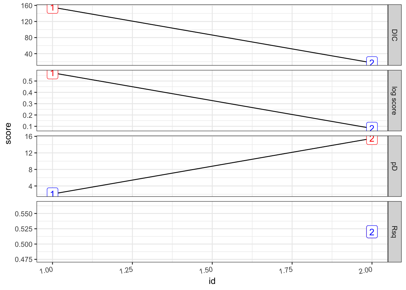
# Sumamry
summary(test_pv_2[[2]])
##
## Call:
## c("inla(formula = formula, family = \"gaussian\", data = dat1, verbose
## = F, ", " control.compute = list(config = T, dic = T, cpo = T, waic =
## T), ", " control.predictor = list(link = 1, compute = TRUE),
## control.fixed = list(correlation.matrix = T))" )
## Time used:
## Pre = 4.74, Running = 0.477, Post = 0.198, Total = 5.42
## Fixed effects:
## mean sd 0.025quant 0.5quant 0.975quant mode kld
## (Intercept) 1.192 1.093 -0.952 1.188 3.353 1.179 0
## viirs 0.177 0.120 -0.059 0.177 0.411 0.178 0
## tmmx -0.044 0.028 -0.099 -0.044 0.011 -0.044 0
## pr 0.000 0.000 0.000 0.000 0.000 0.000 0
##
## Linear combinations (derived):
## ID mean sd 0.025quant 0.5quant 0.975quant mode kld
## (Intercept) 1 1.192 1.093 -0.952 1.188 3.353 1.179 0
## viirs 2 0.177 0.120 -0.059 0.177 0.411 0.178 0
## tmmx 3 -0.044 0.028 -0.099 -0.044 0.011 -0.044 0
## pr 4 0.000 0.000 0.000 0.000 0.000 0.000 0
##
## Random effects:
## Name Model
## index BYM model
## Year IID model
##
## Model hyperparameters:
## mean sd 0.025quant 0.5quant
## Precision for the Gaussian observations 17.24 2.31 13.08 17.12
## Precision for index (iid component) 2203.38 2143.32 233.12 1585.39
## Precision for index (spatial component) 199.58 228.73 28.74 131.01
## Precision for Year 11.10 8.38 1.84 8.99
## 0.975quant mode
## Precision for the Gaussian observations 22.14 16.90
## Precision for index (iid component) 7896.41 649.00
## Precision for index (spatial component) 788.03 67.15
## Precision for Year 33.01 5.06
##
## Expected number of effective parameters(stdev): 13.88(3.62)
## Number of equivalent replicates : 9.72
##
## Deviance Information Criterion (DIC) ...............: 17.24
## Deviance Information Criterion (DIC, saturated) ....: -117.20
## Effective number of parameters .....................: 15.51
##
## Watanabe-Akaike information criterion (WAIC) ...: 20.92
## Effective number of parameters .................: 16.94
##
## Marginal log-Likelihood: -53.91
## CPO and PIT are computed
##
## Posterior marginals for the linear predictor and
## the fitted values are computed(rm_pv_1 <- test_pv_2[[2]] %>% plot_random_map2(map = area.bs, name= "", id = cod, col1 = "gray"))