Chapter 3 Model
3.1 Data
rm(list=ls())
library(tidyverse)
library(purrr)
load("./_dat/NL_VEN_dat.RData")

# d_v_yy <- d_v_yy %>%
#   inner_join(read.csv("./_dat/env_covar.csv"),
#              by = c("ADM2_ES", "ADM3_ES", "Year"))

dat.n <- d_v_yy %>%
  nest(data = everything()) %>%
  crossing(id=1:45) %>%
  mutate(dat_subset = purrr::map2(.x = data, .y = id, .f = ~filter(.x, id!=.y)))

#a <- dat.n$dat_subset[[3]]
3.2 Random Effects
2 methods evaluated: - Zero-inflated Negative binomial regression - Zero-inflated Poisson regression
library(glmmTMB)
library(lme4)
library(pscl)

dat.n <- dat.n %>%
  mutate(fit_ziNB = purrr::map(.x = dat_subset,
                               .f = ~glmmTMB(PV ~ viirs + mei + (1 | id) + offset(log(pop)),
                                             data=.x, ziformula=~1, family="nbinom2")),
         fit_ziPOIS = purrr::map(.x = dat_subset,
                               .f = ~zeroinfl(PV ~ viirs + mei + offset(log(pop)) | id,
                                              data = .x)))


dat.n2 <- dat.n %>%
  mutate(summ_NB = purrr::map(.x = fit_ziNB, .f = ~summary(.x)),
         est_NB = purrr::map(.x = summ_NB, .f = ~coefficients(.x)$cond %>% as.data.frame() %>%
                               rownames_to_column("name") %>% filter(name == "viirs") %>%
                               setNames(paste0('ziNB.', names(.)))),
         summ_POIS = purrr::map(.x = fit_ziPOIS, .f = ~summary(.x)),
         est_POIS = purrr::map(.x = summ_POIS, .f = ~coefficients(.x)$count %>% as.data.frame() %>%
                               rownames_to_column("name") %>% filter(name == "viirs") %>%
                               setNames(paste0('ziPOIS.', names(.)))))

results <- dat.n2 %>%
  dplyr::select(id, est_NB, est_POIS) %>%
  unnest()

#fit_ziNB <- glmmTMB(PV ~ viirs + (1 | id) + offset(log(pop)), data=d_v_yy, ziformula=~1, family="nbinom2")
#summary(fit_ziNB)
results %>%
ggplot(aes(`ziNB.Pr(>|z|)`)) +
geom_histogram() +
geom_vline(xintercept = .05, linetype="dashed") +
labs(title = "Histogram p-value Zero-inflated (ZI) Negative Binomial model") +
theme_bw()
results %>%
  ggplot(aes(`ziPOIS.Pr(>|z|)`)) +
  geom_histogram() +
  geom_vline(xintercept = .05, linetype="dashed") +
  labs(title = "Histogram p-value Zero-inflated (ZI) Poisson model") +
  theme_bw()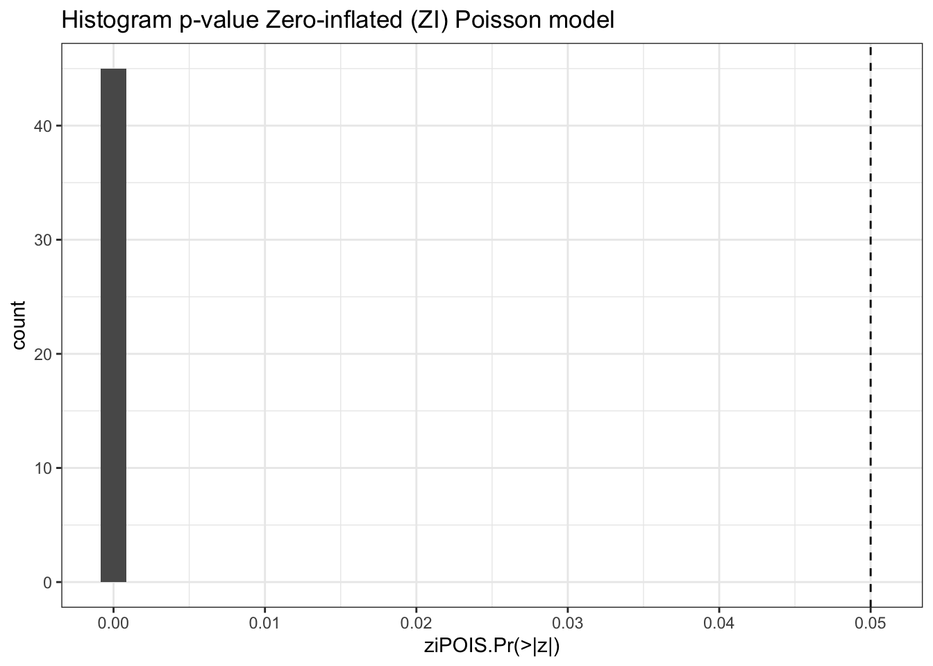
results %>%
  ggplot(aes(x = ziNB.Estimate, y = ziPOIS.Estimate)) +
  #geom_point() +
  geom_smooth(method = "lm", col = "red", fill="red") +
  geom_label(aes(label = id), fill=NA, size = 2) +
  labs(title = "Correlation estimates ZI Poisson ana NEgative Binomial models") +
  theme_bw()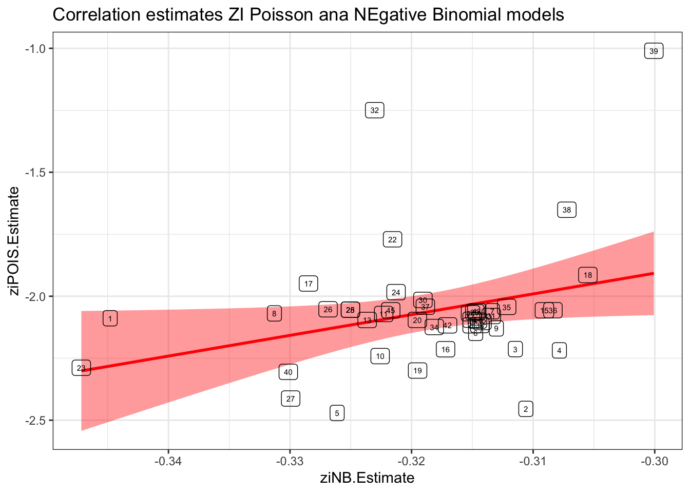
3.3 Bayesian Spatio-temporal
3.3.1 Functions
library(INLA)
library(spdep)
library(purrr)
devtools::source_gist("https://gist.github.com/gcarrascoe/89e018d99bad7d3365ec4ac18e3817bd")

inla.batch <- function(formula, dat1 = dt_final) {
  result = inla(formula, data=dat1, family="nbinomial", offset=log(pop), verbose = F,
                #control.inla=list(strategy="gaussian"),
                control.compute=list(config=T, dic=T, cpo=T, waic=T),
                control.fixed = list(correlation.matrix=T),
                control.predictor=list(link=1,compute=TRUE)
                )
  return(result)
}

inla.batch.safe <- possibly(inla.batch, otherwise = NA_real_)
3.3.2 P. vivax
#Create adjacency matrix
n <- nrow(dt_final)
nb.map <- poly2nb(area.bs)
nb2INLA("./map.graph",nb.map)
codes<-as.data.frame(area.bs)
codes$index<-as.numeric(row.names(codes))
codes<-subset(codes,select=c("cod","index"))
dt_final <- merge(d_v_yy,codes,by="cod") %>%
group_by(index) %>%
mutate(mei = scale_this(mei),
tmmx = scale_this(tmmx),
pr = scale_this(pr))
# MODEL
pv_2<-c(formula = PV ~ 1,
formula = PV ~ 1 + f(index, model = "bym", graph = "./map.graph") +
f(Year, model = "iid") + viirs + mei,
formula = PV ~ 1 + f(index, model = "bym", graph = "./map.graph") +
f(Year, model = "iid") + f(inla.group(viirs), model = "rw1") + mei,
formula = PV ~ 1 + f(index, model = "bym", graph = "./map.graph") +
f(Year, model = "iid") + f(inla.group(viirs), model = "rw1") + tmmx,
formula = PV ~ 1 + f(index, model = "bym", graph = "./map.graph") +
f(Year, model = "iid") + f(inla.group(viirs), model = "rw1") + pr,
formula = PV ~ 1 + f(index, model = "bym", graph = "./map.graph") +
f(Year, model = "iid") + f(inla.group(viirs), model = "rw1") + mei + tmmx + pr)
# ------------------------------------------
# PV estimation
# ------------------------------------------
names(pv_2)<-pv_2
INLA:::inla.dynload.workaround()
test_pv_2 <- pv_2 %>% purrr::map(~inla.batch.safe(formula = .))
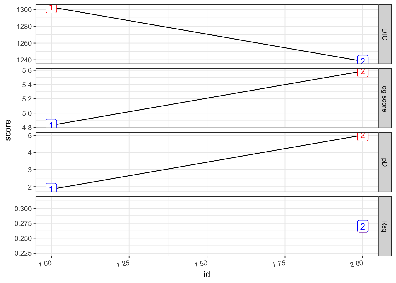
(pv_2.s <- test_pv_2 %>%
purrr::map(~Rsq.batch.safe(model = ., dic.null = test_pv_2[[1]]$dic, n = n)) %>%
bind_rows(.id = "formula") %>% mutate(id = row_number()))
pv_2.s %>%
plot_score()##
## Call:
## c("inla(formula = formula, family = \"nbinomial\", data = dat1, offset
## = log(pop), ", " verbose = F, control.compute = list(config = T, dic =
## T, ", " cpo = T, waic = T), control.predictor = list(link = 1, ", "
## compute = TRUE), control.fixed = list(correlation.matrix = T))" )
## Time used:
## Pre = 1.47, Running = 2.86, Post = 0.104, Total = 4.44
## Fixed effects:
## mean sd 0.025quant 0.5quant 0.975quant mode kld
## (Intercept) -7.286 0.802 -8.880 -7.285 -5.699 -7.284 0
## viirs -0.301 0.043 -0.388 -0.300 -0.218 -0.299 0
## mei 0.006 0.136 -0.262 0.006 0.271 0.007 0
##
## Linear combinations (derived):
## ID mean sd 0.025quant 0.5quant 0.975quant mode kld
## (Intercept) 1 -7.285 0.802 -8.879 -7.284 -5.699 -7.283 0
## viirs 2 -0.301 0.043 -0.387 -0.301 -0.217 -0.300 0
## mei 3 0.005 0.135 -0.261 0.005 0.271 0.006 0
##
## Random effects:
## Name Model
## index BYM model
## Year IID model
##
## Model hyperparameters:
## mean sd
## size for the nbinomial observations (1/overdispersion) 0.838 0.093
## Precision for index (iid component) 0.120 0.021
## Precision for index (spatial component) 1927.593 1888.403
## Precision for Year 0.677 0.412
## 0.025quant 0.5quant
## size for the nbinomial observations (1/overdispersion) 0.685 0.827
## Precision for index (iid component) 0.081 0.120
## Precision for index (spatial component) 127.340 1370.516
## Precision for Year 0.155 0.591
## 0.975quant mode
## size for the nbinomial observations (1/overdispersion) 1.048 0.799
## Precision for index (iid component) 0.164 0.120
## Precision for index (spatial component) 6888.504 346.195
## Precision for Year 1.715 0.405
##
## Expected number of effective parameters(stdev): 48.34(0.298)
## Number of equivalent replicates : 4.65
##
## Deviance Information Criterion (DIC) ...............: 2095.18
## Deviance Information Criterion (DIC, saturated) ....: NaN
## Effective number of parameters .....................: 41.64
##
## Watanabe-Akaike information criterion (WAIC) ...: 2097.13
## Effective number of parameters .................: 35.35
##
## Marginal log-Likelihood: -1141.07
## CPO and PIT are computed
##
## Posterior marginals for the linear predictor and
## the fitted values are computed##
## Call:
## c("inla(formula = formula, family = \"nbinomial\", data = dat1, offset
## = log(pop), ", " verbose = F, control.compute = list(config = T, dic =
## T, ", " cpo = T, waic = T), control.predictor = list(link = 1, ", "
## compute = TRUE), control.fixed = list(correlation.matrix = T))" )
## Time used:
## Pre = 1.61, Running = 4, Post = 0.109, Total = 5.71
## Fixed effects:
## mean sd 0.025quant 0.5quant 0.975quant mode kld
## (Intercept) -13.357 0.971 -15.278 -13.354 -11.454 -13.350 0
## mei 0.021 0.132 -0.239 0.022 0.281 0.022 0
##
## Linear combinations (derived):
## ID mean sd 0.025quant 0.5quant 0.975quant mode kld
## (Intercept) 1 -13.358 0.971 -15.275 -13.356 -11.452 -13.355 0
## mei 2 0.021 0.132 -0.238 0.021 0.281 0.021 0
##
## Random effects:
## Name Model
## index BYM model
## Year IID model
## inla.group(viirs) RW1 model
##
## Model hyperparameters:
## mean sd
## size for the nbinomial observations (1/overdispersion) 0.800 0.089
## Precision for index (iid component) 0.091 0.035
## Precision for index (spatial component) 2034.067 1982.316
## Precision for Year 0.715 0.448
## Precision for inla.group(viirs) 2.688 1.756
## 0.025quant 0.5quant
## size for the nbinomial observations (1/overdispersion) 0.657 0.788
## Precision for index (iid component) 0.031 0.090
## Precision for index (spatial component) 96.216 1430.590
## Precision for Year 0.125 0.628
## Precision for inla.group(viirs) 0.644 2.266
## 0.975quant mode
## size for the nbinomial observations (1/overdispersion) 1.003 0.758
## Precision for index (iid component) 0.159 0.081
## Precision for index (spatial component) 7240.345 227.204
## Precision for Year 1.801 0.371
## Precision for inla.group(viirs) 7.216 1.554
##
## Expected number of effective parameters(stdev): 53.99(1.12)
## Number of equivalent replicates : 4.17
##
## Deviance Information Criterion (DIC) ...............: 2098.00
## Deviance Information Criterion (DIC, saturated) ....: NaN
## Effective number of parameters .....................: 41.76
##
## Watanabe-Akaike information criterion (WAIC) ...: 2106.36
## Effective number of parameters .................: 40.55
##
## Marginal log-Likelihood: -1144.78
## CPO and PIT are computed
##
## Posterior marginals for the linear predictor and
## the fitted values are computed##
## Call:
## c("inla(formula = formula, family = \"nbinomial\", data = dat1, offset
## = log(pop), ", " verbose = F, control.compute = list(config = T, dic =
## T, ", " cpo = T, waic = T), control.predictor = list(link = 1, ", "
## compute = TRUE), control.fixed = list(correlation.matrix = T))" )
## Time used:
## Pre = 1.67, Running = 4.32, Post = 0.111, Total = 6.1
## Fixed effects:
## mean sd 0.025quant 0.5quant 0.975quant mode kld
## (Intercept) -13.147 0.989 -15.178 -13.119 -11.270 -13.063 0
## mei 0.074 0.135 -0.194 0.074 0.338 0.075 0
## tmmx 0.876 0.131 0.621 0.875 1.135 0.873 0
## pr 1.005 0.108 0.794 1.005 1.218 1.004 0
##
## Linear combinations (derived):
## ID mean sd 0.025quant 0.5quant 0.975quant mode kld
## (Intercept) 1 -13.148 0.989 -15.174 -13.121 -11.269 -13.064 0
## mei 2 0.073 0.135 -0.193 0.073 0.339 0.073 0
## tmmx 3 0.876 0.131 0.621 0.875 1.134 0.873 0
## pr 4 1.005 0.108 0.793 1.005 1.218 1.005 0
##
## Random effects:
## Name Model
## index BYM model
## Year IID model
## inla.group(viirs) RW1 model
##
## Model hyperparameters:
## mean sd
## size for the nbinomial observations (1/overdispersion) 8.53e-01 1.48e-01
## Precision for index (iid component) 1.03e-01 3.00e-02
## Precision for index (spatial component) 2.04e+03 1.97e+03
## Precision for Year 1.80e+04 1.88e+04
## Precision for inla.group(viirs) 2.38e+00 1.95e+00
## 0.025quant 0.5quant
## size for the nbinomial observations (1/overdispersion) 0.555 8.61e-01
## Precision for index (iid component) 0.062 9.80e-02
## Precision for index (spatial component) 109.257 1.45e+03
## Precision for Year 1256.914 1.24e+04
## Precision for inla.group(viirs) 0.170 1.87e+00
## 0.975quant mode
## size for the nbinomial observations (1/overdispersion) 1.12e+00 0.897
## Precision for index (iid component) 1.77e-01 0.087
## Precision for index (spatial component) 7.18e+03 274.384
## Precision for Year 6.83e+04 3449.527
## Precision for inla.group(viirs) 7.22e+00 0.471
##
## Expected number of effective parameters(stdev): 51.78(1.77)
## Number of equivalent replicates : 4.34
##
## Deviance Information Criterion (DIC) ...............: 2121.29
## Deviance Information Criterion (DIC, saturated) ....: NaN
## Effective number of parameters .....................: 52.59
##
## Watanabe-Akaike information criterion (WAIC) ...: 2122.02
## Effective number of parameters .................: 42.94
##
## Marginal log-Likelihood: -1142.11
## CPO and PIT are computed
##
## Posterior marginals for the linear predictor and
## the fitted values are computed


3.3.3 P. falciparum
# MODEL
pf_2<-c(formula = PF ~ 1,
        formula = PF ~ 1 + f(index, model = "bym", graph = "./map.graph") +
          f(Year, model = "iid") + viirs + mei,
        formula = PF ~ 1 + f(index, model = "bym", graph = "./map.graph") +
          f(Year, model = "iid") + f(inla.group(viirs), model = "rw1") + mei,
        formula = PF ~ 1 + f(index, model = "bym", graph = "./map.graph") +
          f(Year, model = "iid") + f(inla.group(viirs), model = "rw1") + tmmx,
        formula = PF ~ 1 + f(index, model = "bym", graph = "./map.graph") +
          f(Year, model = "iid") + f(inla.group(viirs), model = "rw1") + pr,
        formula = PF ~ 1 + f(index, model = "bym", graph = "./map.graph") +
          f(Year, model = "iid") + f(inla.group(viirs), model = "rw1") + mei + tmmx + pr)

# ------------------------------------------
# PV estimation
# ------------------------------------------
names(pf_2)<-pf_2

INLA:::inla.dynload.workaround()
test_pf_2 <- pf_2 %>% purrr::map(~inla.batch.safe(formula = .))

(pf_2.s <- test_pf_2 %>%
  purrr::map(~Rsq.batch.safe(model = ., dic.null = test_pf_2[[1]]$dic, n = n)) %>%
  bind_rows(.id = "formula") %>% mutate(id = row_number()))

pf_2.s %>%
plot_score()##
## Call:
## c("inla(formula = formula, family = \"nbinomial\", data = dat1, offset
## = log(pop), ", " verbose = F, control.compute = list(config = T, dic =
## T, ", " cpo = T, waic = T), control.predictor = list(link = 1, ", "
## compute = TRUE), control.fixed = list(correlation.matrix = T))" )
## Time used:
## Pre = 1.45, Running = 1.26, Post = 0.102, Total = 2.82
## Fixed effects:
## mean sd 0.025quant 0.5quant 0.975quant mode kld
## (Intercept) -8.989 0.795 -10.571 -8.986 -7.426 -8.981 0
## viirs -0.346 0.063 -0.479 -0.344 -0.229 -0.338 0
## mei 0.098 0.135 -0.171 0.098 0.361 0.100 0
##
## Linear combinations (derived):
## ID mean sd 0.025quant 0.5quant 0.975quant mode kld
## (Intercept) 1 -8.989 0.795 -10.571 -8.986 -7.426 -8.980 0
## viirs 2 -0.346 0.064 -0.474 -0.345 -0.224 -0.343 0
## mei 3 0.098 0.135 -0.169 0.098 0.362 0.098 0
##
## Random effects:
## Name Model
## index BYM model
## Year IID model
##
## Model hyperparameters:
## mean sd
## size for the nbinomial observations (1/overdispersion) 1.10 0.155
## Precision for index (iid component) 0.08 0.020
## Precision for index (spatial component) 1824.02 1809.050
## Precision for Year 1.06 0.668
## 0.025quant 0.5quant
## size for the nbinomial observations (1/overdispersion) 0.827 1.093
## Precision for index (iid component) 0.047 0.078
## Precision for index (spatial component) 124.003 1289.305
## Precision for Year 0.243 0.917
## 0.975quant mode
## size for the nbinomial observations (1/overdispersion) 1.437 1.074
## Precision for index (iid component) 0.125 0.075
## Precision for index (spatial component) 6631.656 339.028
## Precision for Year 2.759 0.624
##
## Expected number of effective parameters(stdev): 46.69(0.386)
## Number of equivalent replicates : 4.82
##
## Deviance Information Criterion (DIC) ...............: 1540.12
## Deviance Information Criterion (DIC, saturated) ....: NaN
## Effective number of parameters .....................: 46.43
##
## Watanabe-Akaike information criterion (WAIC) ...: 1534.77
## Effective number of parameters .................: 33.39
##
## Marginal log-Likelihood: -854.28
## CPO and PIT are computed
##
## Posterior marginals for the linear predictor and
## the fitted values are computed##
## Call:
## c("inla(formula = formula, family = \"nbinomial\", data = dat1, offset
## = log(pop), ", " verbose = F, control.compute = list(config = T, dic =
## T, ", " cpo = T, waic = T), control.predictor = list(link = 1, ", "
## compute = TRUE), control.fixed = list(correlation.matrix = T))" )
## Time used:
## Pre = 1.63, Running = 3.98, Post = 0.107, Total = 5.71
## Fixed effects:
## mean sd 0.025quant 0.5quant 0.975quant mode kld
## (Intercept) -16.041 1.302 -18.674 -16.019 -13.557 -15.988 0
## mei 0.096 0.136 -0.174 0.097 0.362 0.099 0
##
## Linear combinations (derived):
## ID mean sd 0.025quant 0.5quant 0.975quant mode kld
## (Intercept) 1 -16.041 1.301 -18.645 -16.028 -13.536 -16.014 0
## mei 2 0.096 0.136 -0.172 0.096 0.363 0.097 0
##
## Random effects:
## Name Model
## index BYM model
## Year IID model
## inla.group(viirs) RW1 model
##
## Model hyperparameters:
## mean sd
## size for the nbinomial observations (1/overdispersion) 0.935 0.116
## Precision for index (iid component) 0.089 0.023
## Precision for index (spatial component) 1621.490 1816.504
## Precision for Year 1.109 0.683
## Precision for inla.group(viirs) 2.222 2.249
## 0.025quant 0.5quant
## size for the nbinomial observations (1/overdispersion) 0.747 0.920
## Precision for index (iid component) 0.051 0.087
## Precision for index (spatial component) 107.629 1069.885
## Precision for Year 0.240 0.967
## Precision for inla.group(viirs) 0.441 1.547
## 0.975quant mode
## size for the nbinomial observations (1/overdispersion) 1.20 0.884
## Precision for index (iid component) 0.14 0.082
## Precision for index (spatial component) 6478.80 292.022
## Precision for Year 2.83 0.644
## Precision for inla.group(viirs) 8.05 0.905
##
## Expected number of effective parameters(stdev): 51.52(1.23)
## Number of equivalent replicates : 4.37
##
## Deviance Information Criterion (DIC) ...............: 1539.77
## Deviance Information Criterion (DIC, saturated) ....: NaN
## Effective number of parameters .....................: 43.33
##
## Watanabe-Akaike information criterion (WAIC) ...: 1539.23
## Effective number of parameters .................: 34.67
##
## Marginal log-Likelihood: -856.70
## CPO and PIT are computed
##
## Posterior marginals for the linear predictor and
## the fitted values are computed##
## Call:
## c("inla(formula = formula, family = \"nbinomial\", data = dat1, offset
## = log(pop), ", " verbose = F, control.compute = list(config = T, dic =
## T, ", " cpo = T, waic = T), control.predictor = list(link = 1, ", "
## compute = TRUE), control.fixed = list(correlation.matrix = T))" )
## Time used:
## Pre = 1.68, Running = 4.24, Post = 0.11, Total = 6.03
## Fixed effects:
## mean sd 0.025quant 0.5quant 0.975quant mode kld
## (Intercept) -15.784 1.179 -18.230 -15.743 -13.575 -15.667 0
## mei 0.018 0.141 -0.260 0.019 0.294 0.020 0
## tmmx 0.658 0.142 0.381 0.657 0.938 0.656 0
## pr 0.867 0.113 0.648 0.866 1.093 0.864 0
##
## Linear combinations (derived):
## ID mean sd 0.025quant 0.5quant 0.975quant mode kld
## (Intercept) 1 -15.784 1.179 -18.204 -15.751 -13.551 -15.688 0
## mei 2 0.018 0.141 -0.259 0.018 0.294 0.019 0
## tmmx 3 0.658 0.142 0.381 0.657 0.938 0.656 0
## pr 4 0.867 0.113 0.647 0.867 1.091 0.866 0
##
## Random effects:
## Name Model
## index BYM model
## Year IID model
## inla.group(viirs) RW1 model
##
## Model hyperparameters:
## mean sd
## size for the nbinomial observations (1/overdispersion) 1.19e+00 1.26e-01
## Precision for index (iid component) 8.80e-02 2.20e-02
## Precision for index (spatial component) 1.59e+03 1.83e+03
## Precision for Year 1.99e+04 1.94e+04
## Precision for inla.group(viirs) 2.17e+00 1.50e+00
## 0.025quant 0.5quant
## size for the nbinomial observations (1/overdispersion) 0.941 1.19e+00
## Precision for index (iid component) 0.051 8.70e-02
## Precision for index (spatial component) 103.023 1.03e+03
## Precision for Year 1247.772 1.42e+04
## Precision for inla.group(viirs) 0.427 1.82e+00
## 0.975quant mode
## size for the nbinomial observations (1/overdispersion) 1.43e+00 1.206
## Precision for index (iid component) 1.38e-01 0.083
## Precision for index (spatial component) 6.46e+03 279.243
## Precision for Year 7.09e+04 3317.616
## Precision for inla.group(viirs) 6.03e+00 1.134
##
## Expected number of effective parameters(stdev): 49.27(1.12)
## Number of equivalent replicates : 4.57
##
## Deviance Information Criterion (DIC) ...............: 1556.59
## Deviance Information Criterion (DIC, saturated) ....: 277.32
## Effective number of parameters .....................: 50.55
##
## Watanabe-Akaike information criterion (WAIC) ...: 1549.09
## Effective number of parameters .................: 34.87
##
## Marginal log-Likelihood: -855.23
## CPO and PIT are computed
##
## Posterior marginals for the linear predictor and
## the fitted values are computed