Chapter 5 Mediation Analysis 4-way decompositon
5.1 Data
rm(list = ls())
library(tidyverse)
library(kableExtra)
library(jtools)
library(sf)
load("./_data/rscd_jr.RData")

dat <- d2 %>%
  dplyr::select(id_house, comm, id_study:viaje_ult_mes,SEROPOSITIVE, main_act_ec:fumigacion, area) %>%
  st_set_geometry(NULL) %>%
  mutate(viaje_ult_mes = ifelse(viaje_ult_mes=="9999", NA, viaje_ult_mes),
         viaje_ult_mes = factor(ifelse(viaje_ult_mes=="2", "1_yes", "0_no")),
         SEROPOSITIVE = ifelse(SEROPOSITIVE=="Positive",1,0),
         work_out = factor(ifelse(as.numeric(main_act_ec)>0 & as.numeric(main_act_ec)<6, "outside", "inside"))) #%>% filter(complete.cases(.))

dat_gf_1 <- dat %>%
  #dplyr::select(viaje_ult_mes, work_out, edad, SEROPOSITIVE, nm_sex, comm, area) %>%
  mutate(id = seq(1:n()),
         time = 0,
         viaje_ult_mes = as.integer(as.numeric(viaje_ult_mes)-1),
         work_out = as.numeric(work_out)-1,
         sex_male = as.numeric(nm_sex)-1,
         SEROPOSITIVE = as.integer(SEROPOSITIVE),
         edad = as.numeric(edad)#,
         #edad = edad*edad
         ) %>%
  #filter(complete.cases(.)) %>%
  as.data.frame()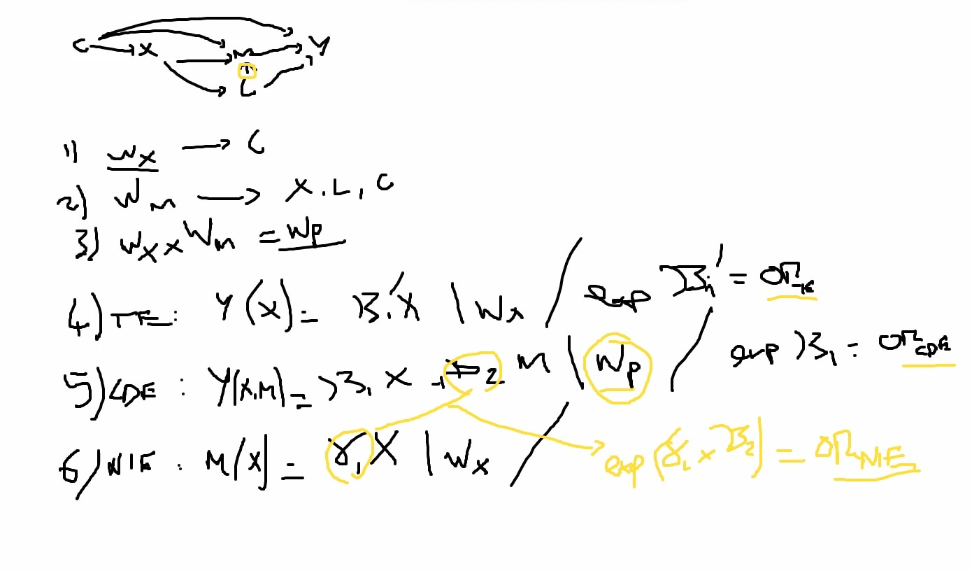
5.2 Weights
#C = edad
#X = sex_male
#M = work_out
#L = viaje_ult_mes
#Y = SEROPOSITIVE

#p1 <- glm(sex_male ~ ... , data = dat_gf, family = "binomial")
dat_gf_2 <- dat_gf_1 %>%
  mutate(wx = 1,
         tipo_casa = factor(tipo_casa)) #%>%
  # mutate(ps1 = predict(p1, type = "response"),
  #        wx = ifelse(sex_male==1, 1/ps1, 1/(1-ps1)))
p <- glm(work_out ~ 1, data = dat_gf_2, family = "binomial")

p2 <- glm(work_out ~ (sex_male + edad + fumigacion + animales_casa + tipo_casa)^2,
          data = dat_gf_2, family = "binomial")

dat_gf <- dat_gf_2 %>%
  mutate(p = predict(p, type="response"),
         ps2 = predict(p2, type = "response"),
         wm = ifelse(work_out==1, p/ps2, p/(1-ps2)),
         wp = wm*wx)

dat_gf %>%
  ggplot(aes(x=ps2, fill= factor(work_out))) +
  geom_density(alpha=.5) +
  #scale_x_continuous(trans = "log10") +
  theme_nice() +
  theme(legend.position = "top")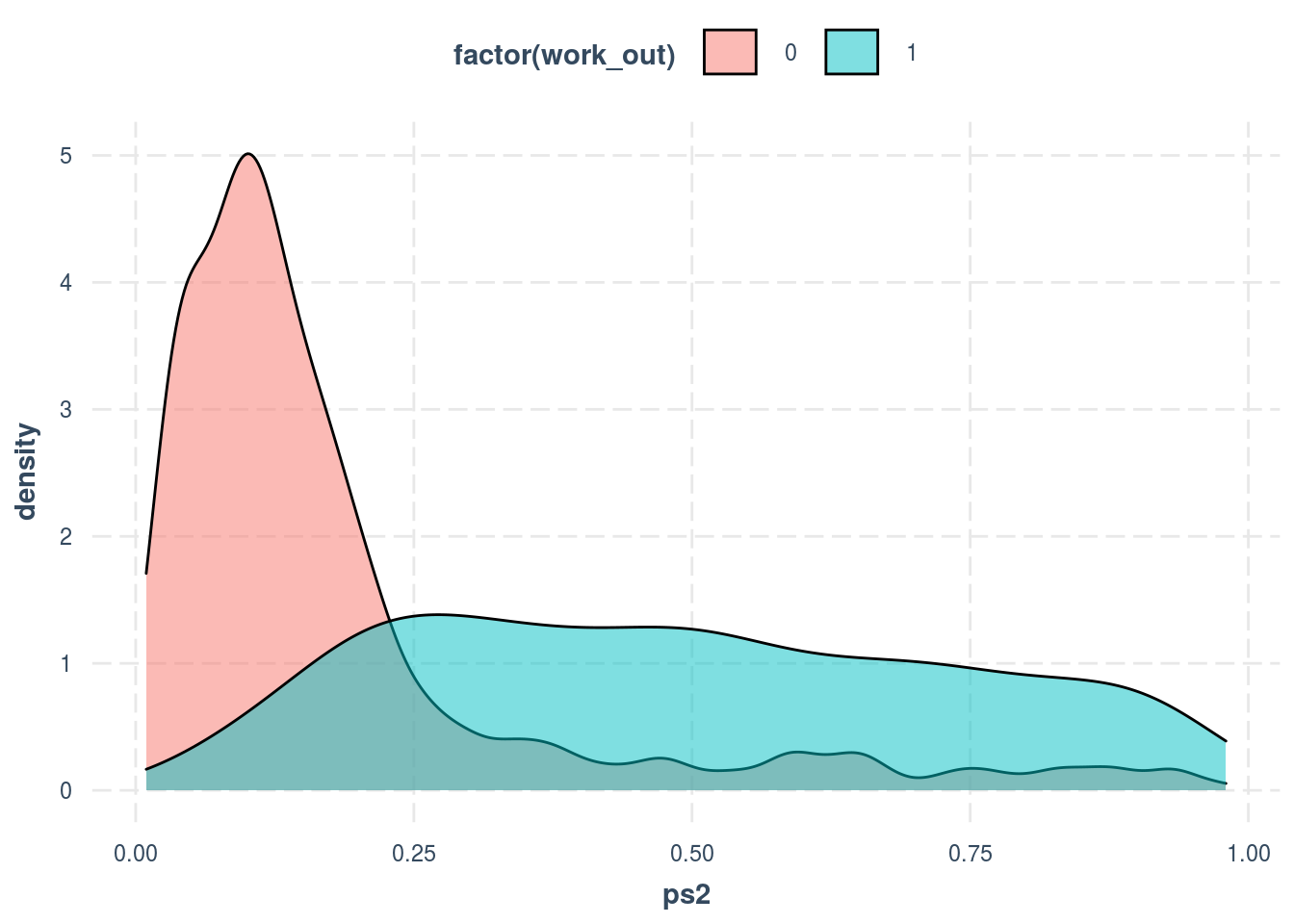
## # A tibble: 2 x 3
##   work_out     m    sd
##      <dbl> <dbl> <dbl>
## 1        0 0.185 0.192
## 2        1 0.496 0.246
# LOVE PLOT
library(cobalt)
library(WeightIt)
w.out1 <- weightit(work_out ~ (sex_male + edad + fumigacion + animales_casa + tipo_casa)^2,
data = dat_gf_2, estimand = "ATE", method = "ps")
love.plot(w.out1)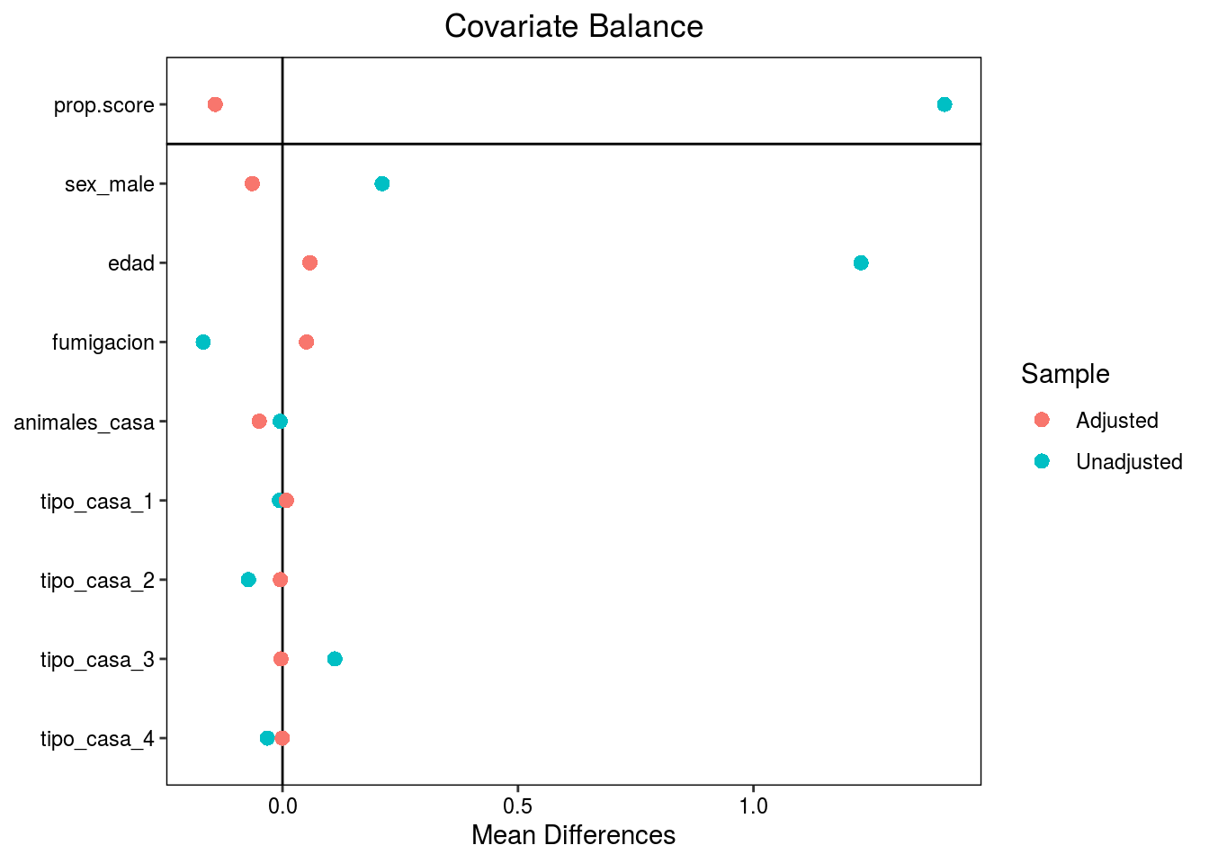
5.3 Hand calculation
5.3.1 outcome regression
eq1 <- glm(SEROPOSITIVE ~ sex_male*work_out + comm, weights = wp, data = dat_gf, family = "binomial")
(summ.eq1 <- summ(eq1, confint = T))| Observations | 1790 |
| Dependent variable | SEROPOSITIVE |
| Type | Generalized linear model |
| Family | binomial |
| Link | logit |
| 𝛘²(12) | 215.77 |
| Pseudo-R² (Cragg-Uhler) | 0.20 |
| Pseudo-R² (McFadden) | 0.18 |
| AIC | 605.90 |
| BIC | 677.27 |
| Est. | 2.5% | 97.5% | z val. | p | |
|---|---|---|---|---|---|
| (Intercept) | -1.05 | -1.52 | -0.58 | -4.40 | 0.00 |
| sex_male | 0.39 | 0.02 | 0.75 | 2.09 | 0.04 |
| work_out | 1.28 | 0.84 | 1.73 | 5.65 | 0.00 |
| comm502 | 1.52 | 0.97 | 2.07 | 5.42 | 0.00 |
| comm503 | -0.04 | -0.62 | 0.54 | -0.14 | 0.89 |
| comm901 | 2.98 | 1.38 | 4.59 | 3.64 | 0.00 |
| comm902 | 2.03 | 1.33 | 2.72 | 5.71 | 0.00 |
| comm903 | 1.17 | 0.24 | 2.10 | 2.46 | 0.01 |
| comm904 | 0.39 | -0.17 | 0.95 | 1.38 | 0.17 |
| comm905 | -0.72 | -1.50 | 0.05 | -1.83 | 0.07 |
| comm906 | 0.33 | -0.28 | 0.94 | 1.06 | 0.29 |
| comm907 | 1.37 | 0.75 | 2.00 | 4.28 | 0.00 |
| sex_male:work_out | 0.11 | -0.52 | 0.73 | 0.33 | 0.74 |
| Standard errors: MLE |
## [1] 0.3889764## [1] 1.281463## [1] 1.5211075.3.2 mediator regression
eq2 <- glm(work_out ~ sex_male + comm, data = dat_gf, weights = wx, family = "binomial")
(summ.eq2 <- summ(eq2, confint = T))| Observations | 1790 |
| Dependent variable | work_out |
| Type | Generalized linear model |
| Family | binomial |
| Link | logit |
| 𝛘²(10) | 335.15 |
| Pseudo-R² (Cragg-Uhler) | 0.25 |
| Pseudo-R² (McFadden) | 0.16 |
| AIC | 1770.33 |
| BIC | 1830.72 |
| Est. | 2.5% | 97.5% | z val. | p | |
|---|---|---|---|---|---|
| (Intercept) | -2.88 | -3.36 | -2.40 | -11.75 | 0.00 |
| sex_male | 0.85 | 0.62 | 1.08 | 7.21 | 0.00 |
| comm502 | 0.79 | 0.22 | 1.35 | 2.73 | 0.01 |
| comm503 | -0.99 | -1.84 | -0.15 | -2.31 | 0.02 |
| comm901 | 2.21 | 1.46 | 2.96 | 5.77 | 0.00 |
| comm902 | 2.15 | 1.60 | 2.71 | 7.67 | 0.00 |
| comm903 | 1.91 | 1.20 | 2.62 | 5.27 | 0.00 |
| comm904 | 2.02 | 1.50 | 2.54 | 7.56 | 0.00 |
| comm905 | 2.12 | 1.50 | 2.73 | 6.72 | 0.00 |
| comm906 | 2.35 | 1.79 | 2.90 | 8.27 | 0.00 |
| comm907 | 1.82 | 1.27 | 2.38 | 6.47 | 0.00 |
| Standard errors: MLE |
## [1] 0.84772655.3.3 Summary
- Do we need to include non-significant betas?? (mediator regression)
## [1] 0.3889764## [1] 17.48383## [1] 1.289483## [1] 1.08633## [1] 20.24862## [1] 0.01921002## [1] 0.8634579## [1] 0.06368252## [1] 0.05364959## [1] 2.375813## [1] 17.87281## [1] 19.16229## [1] 19.85964## [1] 18.773315.4 Package
#-----------------------------------------------------------------------------------------------------------
# All libraries here
library(boot)
library(survival)
library(data.table)
library(foreign)
library(dummies)
#library(GenABEL)
#library(dummies)
#-----------------------------------------------------------------------------------------------------------
# Sources import here

# this script should be run from the same folder where src.R is
source('./4way-decomposition-master/src.R')
#-----------------------------------------------------------------------------------------------------------
# Define your parameters here!!!

#Path to save results
output<-"./Test_results.csv"

#Define variables
A<<-'sex_male'
M<<-'work_out'
Y<<-'SEROPOSITIVE'
COVAR<<-c('comm_502', 'comm_503', 'comm_901', 'comm_902', 'comm_903', 'comm_904', 'comm_905', 'comm_906',
          'comm_907')

#1=binary 0=continuous
outcome=1
mediator=1

#Assign levels for the exposure that are being compared;
#for mstar it is the level at which to compute the CDE and the remainder of the decomposition
a<<-1
astar<<-0
mstar<<-0

#Boostrap number of iterations
N_r=5

#-----------------------------------------------------------------------------------------------------------
####### DONT TOUCH FROM HERE #######
#------------------------------------------------------------------------------------------------------------

# Reading data file
#data<-read.spss(data_path, to.data.frame=T) #TODO spss/csv/txt (?)
data<-dat_gf %>%
  mutate(area = as.numeric(area)) %>%
  fastDummies::dummy_cols(remove_first_dummy = TRUE)

if (! prod(c(A,Y,M,COVAR) %in% names(data) ) )  {stop('Some of defined variable names are not in data file!')}

if ( mediator==1 & outcome==1 ) {  save_results(output=output, boot_function=boot.bMbO, N=N_r)  }
if ( mediator==0 & outcome==1 ) {  save_results(output=output, boot_function=boot.cMbO, N=N_r)  }
if ( mediator==1 & outcome==0 ) {  save_results(output=output, boot_function=boot.bMcO, N=N_r)  }
if ( mediator==0 & outcome==0 ) {  save_results(output=output, boot_function=boot.cMcO, N=N_r)  }


table.4wd <- read.csv("./Test_results.csv")
kable(table.4wd)| X | Estimand | Estimate | LCL | UCL |
|---|---|---|---|---|
| 1 | Total Effect Risk Ratio | 1.9892741 | 1.5116620 | 2.7702863 |
| 2 | Total Excess Relative Risk | 0.9892741 | 0.5116620 | 1.7702863 |
| 3 | Excess Relative Risk due to CDE | 0.3425417 | 0.2614241 | 0.5428315 |
| 4 | Excess Relative Risk due to INTref | 0.1962163 | -0.0053691 | 0.5569330 |
| 5 | Excess Relative Risk due to INTmed | 0.1857939 | -0.0829007 | 0.5382547 |
| 6 | Excess Relative Risk due to PIE | 0.2647221 | 0.1322672 | 0.3385078 |
| 7 | Proportion CDE | 0.3462556 | 0.0094677 | 0.4036958 |
| 8 | Proportion INTref | 0.1983437 | 0.1254996 | 1.1865604 |
| 9 | Proportion INTmed | 0.1878084 | 0.0657845 | 1.1758921 |
| 10 | Proportion PIE | 0.2675923 | -1.3719201 | 0.4050201 |
| 11 | Overall Proportion Mediated | 0.4554006 | -0.1960281 | 0.5021461 |
| 12 | Overall Proportion Attributable to Interaction | 0.3861521 | 0.1912841 | 2.3624524 |
| 13 | Overall Proportion Eliminated | 0.6537444 | 0.5963042 | 0.9905323 |