Chapter 2 Mediation Analysis - The product Method
2.1 Data
rm(list = ls())
library(tidyverse)
library(kableExtra)
library(jtools)
library(sf)
library(broom)
library(pubh)
library(huxtable)
library(robustbase)
source("./causinf_fun.R")

#OPTIONS
options('huxtable.knit_print_df_theme' = theme_article)
options('huxtable.autoformat_number_format' = list(numeric = "%5.2f"))

load("./_data/rscd_jr.RData")

dat <- d2 %>%
  dplyr::select(id_house, comm, id_study:viaje_ult_mes,SEROPOSITIVE, main_act_ec:fumigacion, area) %>%
  st_set_geometry(NULL) %>%
  mutate(viaje_ult_mes = ifelse(viaje_ult_mes=="9999", NA, viaje_ult_mes),
         viaje_ult_mes = factor(ifelse(viaje_ult_mes=="2", "1_yes", "0_no")),
         SEROPOSITIVE = ifelse(SEROPOSITIVE=="Positive",1,0),
         sex_male = as.numeric(nm_sex)-1,
         work_out1 = factor(ifelse(as.numeric(main_act_ec)>0 & as.numeric(main_act_ec)<6, "outside", "inside"))) #%>% filter(complete.cases(.))

dat_gf_1 <- dat %>%
  #dplyr::select(viaje_ult_mes, work_out, edad, SEROPOSITIVE, nm_sex, comm, area) %>%
  mutate(id = seq(1:n()),
         time = 0,
         viaje_ult_mes = as.integer(as.numeric(viaje_ult_mes)-1),
         work_out = as.numeric(work_out1)-1,
         SEROPOSITIVE = as.integer(SEROPOSITIVE),
         edad = as.numeric(edad)#,
         #edad = edad*edad
         ) %>%
  #filter(complete.cases(.)) %>%
  as.data.frame()
2.2 Weights
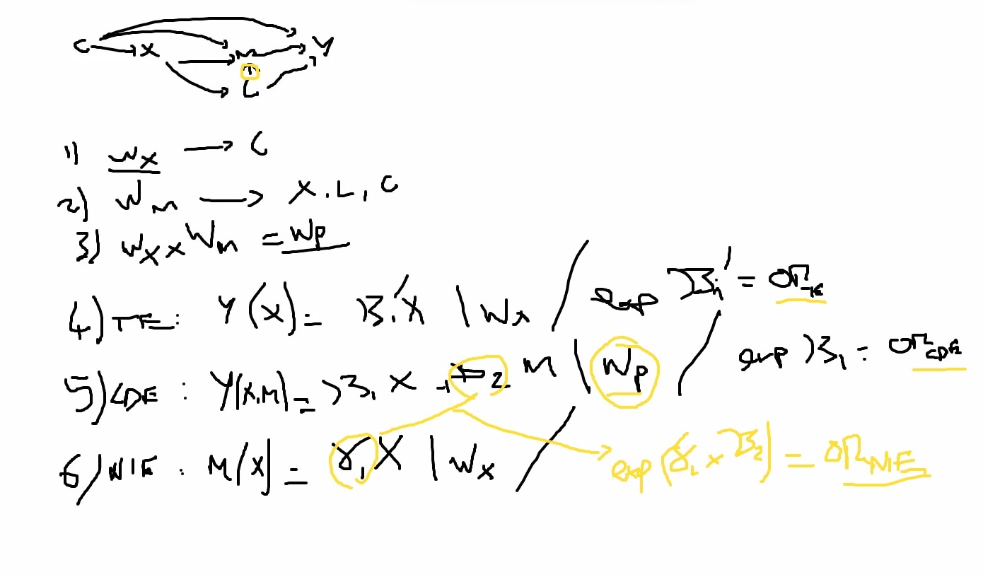
#C = edad
#X = sex_male
#M = work_out
#L = viaje_ult_mes
#Y = SEROPOSITIVE

#p1 <- glm(sex_male ~ ... , data = dat_gf, family = "binomial")
dat_gf_2 <- dat_gf_1 %>%
  mutate(wx = 1,
         tipo_casa = factor(tipo_casa)) #%>%
  # mutate(ps1 = predict(p1, type = "response"),
  #        wx = ifelse(sex_male==1, 1/ps1, 1/(1-ps1)))
p <- glm(work_out ~ 1, data = dat_gf_2, family = "binomial")

p2 <- glm(work_out ~ (sex_male + edad + fumigacion + animales_casa + tipo_casa)^2,
          data = dat_gf_2, family = "binomial")

dat_gf <- dat_gf_2 %>%
  mutate(p = predict(p, type="response"),
         ps2 = predict(p2, type = "response"),
         wm = ifelse(work_out==1, p/ps2, p/(1-ps2)),
         wp = wm*wx)

dat_gf %>%
  ggplot(aes(x=ps2, fill= factor(work_out))) +
  geom_density(alpha=.5) +
  #scale_x_continuous(trans = "log10") +
  theme_nice() +
  theme(legend.position = "top")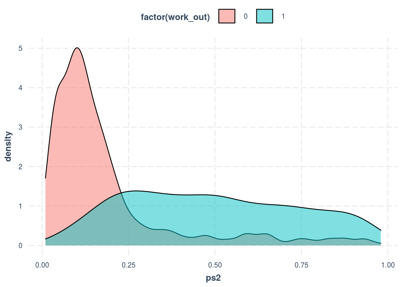
| work_out1 | N | Min. | Max. | Mean | Median | SD | CV | |
|---|---|---|---|---|---|---|---|---|
| ps2 | inside | 1309.00 | 0.01 | 0.98 | 0.19 | 0.12 | 0.19 | 1.04 |
| outside | 481.00 | 0.04 | 0.97 | 0.50 | 0.49 | 0.25 | 0.50 |
# LOVE PLOT
library(cobalt)
library(WeightIt)

w.out1 <- weightit(work_out ~ (sex_male + edad + fumigacion + animales_casa + tipo_casa)^2,
                   data = dat_gf_2, estimand = "ATE", method = "ps")

love.plot(w.out1)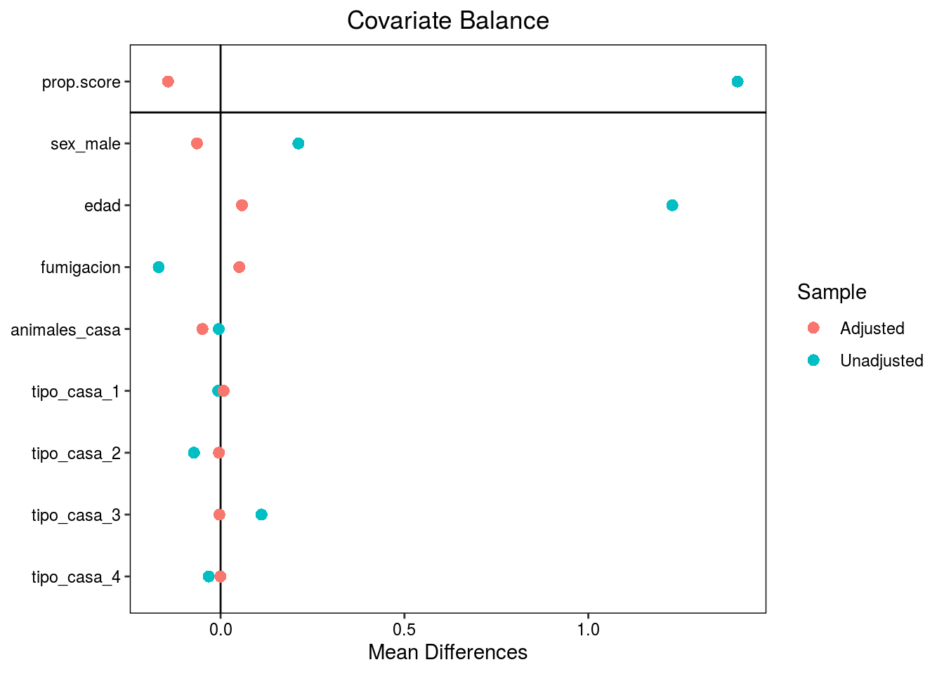
2.3 The product method
References - Mediation Analysis: VanderWeele, 2016 - Regression Model Zou, 2004
2.3.1 Overall
# Total Effect
te <- glmrob(SEROPOSITIVE ~ sex_male + comm, data = dat_gf, weights = wp, family = "poisson")
(te.t <- te %>% tidy(conf.int = T))| term | estimate | std.error | statistic | p.value | conf.low | conf.high |
|---|---|---|---|---|---|---|
| (Intercept) | -1.10 | 0.19 | -5.66 | 0.00 | -1.48 | -0.72 |
| sex_male | -0.10 | 0.11 | -0.92 | 0.36 | -0.32 | 0.11 |
| comm502 | 0.95 | 0.24 | 4.04 | 0.00 | 0.49 | 1.42 |
| comm503 | 0.25 | 0.26 | 0.97 | 0.33 | -0.26 | 0.76 |
| comm901 | 1.02 | 0.30 | 3.40 | 0.00 | 0.43 | 1.61 |
| comm902 | 0.96 | 0.22 | 4.38 | 0.00 | 0.53 | 1.39 |
| comm903 | 0.75 | 0.36 | 2.11 | 0.04 | 0.05 | 1.45 |
| comm904 | 0.26 | 0.26 | 1.01 | 0.31 | -0.24 | 0.76 |
| comm905 | 0.10 | 0.35 | 0.27 | 0.79 | -0.59 | 0.78 |
| comm906 | 0.54 | 0.25 | 2.20 | 0.03 | 0.06 | 1.02 |
| comm907 | 0.77 | 0.23 | 3.29 | 0.00 | 0.31 | 1.23 |
## [1] -0.1012378te <- glm(SEROPOSITIVE ~ sex_male + comm, data = dat_gf, weights = wp, family = "poisson")
(te.t <- summ(te, confint = T, model.fit = F, model.info = F, robust = "HC1"))| Est. | 2.5% | 97.5% | z val. | p | |
|---|---|---|---|---|---|
| (Intercept) | -1.02 | -1.31 | -0.73 | -6.84 | 0.00 |
| sex_male | 0.13 | 0.04 | 0.23 | 2.75 | 0.01 |
| comm502 | 0.58 | 0.28 | 0.87 | 3.82 | 0.00 |
| comm503 | -0.22 | -0.62 | 0.17 | -1.12 | 0.26 |
| comm901 | 0.90 | 0.61 | 1.18 | 6.13 | 0.00 |
| comm902 | 0.81 | 0.52 | 1.09 | 5.54 | 0.00 |
| comm903 | 0.61 | 0.27 | 0.96 | 3.48 | 0.00 |
| comm904 | 0.37 | 0.06 | 0.69 | 2.36 | 0.02 |
| comm905 | -0.23 | -0.70 | 0.24 | -0.95 | 0.34 |
| comm906 | 0.43 | 0.10 | 0.75 | 2.56 | 0.01 |
| comm907 | 0.65 | 0.35 | 0.95 | 4.29 | 0.00 |
| Standard errors: Robust, type = HC1 |
## [1] 0.1323782# Controlled Direct Effect
cde <- glm(SEROPOSITIVE ~ sex_male + work_out + comm, data = dat_gf, weights = wp, family = "poisson")
(cde.t <- summ(cde, confint = T, model.fit = F, model.info = F, robust = "HC1"))| Est. | 2.5% | 97.5% | z val. | p | |
|---|---|---|---|---|---|
| (Intercept) | -1.15 | -1.43 | -0.88 | -8.21 | 0.00 |
| sex_male | 0.13 | 0.04 | 0.23 | 2.73 | 0.01 |
| work_out | 0.41 | 0.30 | 0.52 | 7.35 | 0.00 |
| comm502 | 0.64 | 0.34 | 0.93 | 4.24 | 0.00 |
| comm503 | -0.12 | -0.50 | 0.27 | -0.59 | 0.55 |
| comm901 | 0.75 | 0.45 | 1.06 | 4.83 | 0.00 |
| comm902 | 0.66 | 0.36 | 0.96 | 4.30 | 0.00 |
| comm903 | 0.51 | 0.15 | 0.88 | 2.75 | 0.01 |
| comm904 | 0.26 | -0.07 | 0.58 | 1.56 | 0.12 |
| comm905 | -0.32 | -0.77 | 0.13 | -1.40 | 0.16 |
| comm906 | 0.26 | -0.08 | 0.59 | 1.49 | 0.14 |
| comm907 | 0.57 | 0.26 | 0.88 | 3.59 | 0.00 |
| Standard errors: Robust, type = HC1 |
cde.e <- cde.t$coeftable[2,1]
b2 <- cde.t$coeftable[3,1]

# Natual Indirect Effect
nie <- glm(work_out ~ sex_male + comm, data = dat_gf, weights = wp, family = "poisson")
(nie.t <- summ(nie, confint = T, model.fit = F, model.info = F, robust = "HC1"))| Est. | 2.5% | 97.5% | z val. | p | |
|---|---|---|---|---|---|
| (Intercept) | -1.26 | -1.78 | -0.74 | -4.78 | 0.00 |
| sex_male | -0.02 | -0.16 | 0.13 | -0.21 | 0.83 |
| comm502 | -0.63 | -1.24 | -0.01 | -2.00 | 0.05 |
| comm503 | -1.65 | -2.62 | -0.69 | -3.37 | 0.00 |
| comm901 | 0.80 | 0.23 | 1.37 | 2.75 | 0.01 |
| comm902 | 0.82 | 0.30 | 1.34 | 3.07 | 0.00 |
| comm903 | 0.62 | 0.04 | 1.21 | 2.10 | 0.04 |
| comm904 | 0.70 | 0.18 | 1.22 | 2.66 | 0.01 |
| comm905 | 0.60 | 0.03 | 1.16 | 2.07 | 0.04 |
| comm906 | 0.91 | 0.40 | 1.43 | 3.51 | 0.00 |
| comm907 | 0.54 | -0.01 | 1.10 | 1.91 | 0.06 |
| Standard errors: Robust, type = HC1 |
a1 <- nie.t$coeftable[2,1]
nie.e <- a1*b2

# Summary
data.frame(TE_orig = te.e,
           TE_comp = cde.e + nie.e,
prop_med = (exp(cde.e)*(exp(nie.e)-1))/((exp(cde.e)*exp(nie.e))-1))| TE_orig | TE_comp | prop_med |
|---|---|---|
| 0.13 | 0.13 | -0.06 |
2.3.2 Rural
dat_gf_rural <- dat_gf %>%
  filter(area == "1_rural")

# Total Effect
te_r <- glm(SEROPOSITIVE ~ sex_male + comm, data = dat_gf_rural, weights = wp, family = "poisson")
(te_r.t <- summ(te_r, confint = T, model.fit = F, model.info = F, robust = "HC1"))| Est. | 2.5% | 97.5% | z val. | p | |
|---|---|---|---|---|---|
| (Intercept) | -0.09 | -0.17 | -0.02 | -2.47 | 0.01 |
| sex_male | 0.07 | -0.03 | 0.17 | 1.30 | 0.19 |
| comm902 | -0.09 | -0.17 | -0.00 | -1.99 | 0.05 |
| comm903 | -0.28 | -0.50 | -0.06 | -2.51 | 0.01 |
| comm904 | -0.52 | -0.67 | -0.37 | -6.83 | 0.00 |
| comm905 | -1.12 | -1.50 | -0.74 | -5.74 | 0.00 |
| comm906 | -0.47 | -0.65 | -0.29 | -5.14 | 0.00 |
| comm907 | -0.24 | -0.36 | -0.12 | -3.91 | 0.00 |
| Standard errors: Robust, type = HC1 |
te_r.e <- te_r.t$coeftable[2,1]

# Controlled Direct Effect
cde_r <- glm(SEROPOSITIVE ~ sex_male + work_out + comm, data = dat_gf_rural, weights = wp, family = "poisson")
(cde_r.t <- summ(cde_r, confint = T, model.fit = F, model.info = F, robust = "HC1"))| Est. | 2.5% | 97.5% | z val. | p | |
|---|---|---|---|---|---|
| (Intercept) | -0.47 | -0.61 | -0.33 | -6.69 | 0.00 |
| sex_male | 0.10 | -0.00 | 0.20 | 1.88 | 0.06 |
| work_out | 0.53 | 0.40 | 0.65 | 8.45 | 0.00 |
| comm902 | -0.09 | -0.20 | 0.02 | -1.62 | 0.10 |
| comm903 | -0.23 | -0.48 | 0.03 | -1.76 | 0.08 |
| comm904 | -0.49 | -0.66 | -0.33 | -5.90 | 0.00 |
| comm905 | -1.06 | -1.42 | -0.70 | -5.84 | 0.00 |
| comm906 | -0.50 | -0.69 | -0.32 | -5.46 | 0.00 |
| comm907 | -0.17 | -0.32 | -0.02 | -2.23 | 0.03 |
| Standard errors: Robust, type = HC1 |
cde_r.e <- cde_r.t$coeftable[2,1]
b2_r <- cde_r.t$coeftable[3,1]

# Natual Indirect Effect
nie_r <- glm(work_out ~ sex_male + comm, data = dat_gf_rural, weights = wp, family = "poisson")
(nie_r.t <- summ(nie_r, confint = T, model.fit = F, model.info = F, robust = "HC1"))| Est. | 2.5% | 97.5% | z val. | p | |
|---|---|---|---|---|---|
| (Intercept) | -0.43 | -0.71 | -0.15 | -2.99 | 0.00 |
| sex_male | -0.11 | -0.25 | 0.03 | -1.53 | 0.13 |
| comm902 | 0.02 | -0.29 | 0.33 | 0.15 | 0.88 |
| comm903 | -0.16 | -0.57 | 0.24 | -0.78 | 0.43 |
| comm904 | -0.10 | -0.40 | 0.20 | -0.63 | 0.53 |
| comm905 | -0.19 | -0.57 | 0.19 | -0.97 | 0.33 |
| comm906 | 0.12 | -0.18 | 0.41 | 0.79 | 0.43 |
| comm907 | -0.25 | -0.61 | 0.11 | -1.35 | 0.18 |
| Standard errors: Robust, type = HC1 |
a1_r <- nie_r.t$coeftable[2,1]
nie_r.e <- a1_r*b2_r

# Summary
data.frame(TE_orig = te_r.e,
           TE_comp = cde_r.e + nie_r.e,
prop_med = (exp(cde_r.e)*(exp(nie_r.e)-1))/((exp(cde_r.e)*exp(nie_r.e))-1))| TE_orig | TE_comp | prop_med |
|---|---|---|
| 0.07 | 0.04 | -1.48 |
2.3.3 Periurban
dat_gf_urban <- dat_gf %>%
  filter(area == "0_periurban")

# Total Effect
te_u <- glm(SEROPOSITIVE ~ sex_male + comm, data = dat_gf_urban, weights = wp, family = "poisson")
(te_u.t <- summ(te_u, confint = T, model.fit = F, model.info = F, robust = "HC1"))| Est. | 2.5% | 97.5% | z val. | p | |
|---|---|---|---|---|---|
| (Intercept) | -1.08 | -1.42 | -0.75 | -6.41 | 0.00 |
| sex_male | 0.27 | 0.06 | 0.47 | 2.59 | 0.01 |
| comm502 | 0.55 | 0.27 | 0.84 | 3.78 | 0.00 |
| comm503 | -0.24 | -0.62 | 0.15 | -1.18 | 0.24 |
| Standard errors: Robust, type = HC1 |
te_u.e <- te_u.t$coeftable[2,1]

# Controlled Direct Effect
cde_u <- glm(SEROPOSITIVE ~ sex_male + work_out + comm, data = dat_gf_urban, weights = wp, family = "poisson")
(cde_u.t <- summ(cde_u, confint = T, model.fit = F, model.info = F, robust = "HC1"))| Est. | 2.5% | 97.5% | z val. | p | |
|---|---|---|---|---|---|
| (Intercept) | -1.10 | -1.38 | -0.83 | -7.82 | 0.00 |
| sex_male | 0.26 | 0.04 | 0.48 | 2.31 | 0.02 |
| work_out | 0.08 | -0.25 | 0.41 | 0.49 | 0.63 |
| comm502 | 0.57 | 0.31 | 0.83 | 4.30 | 0.00 |
| comm503 | -0.21 | -0.57 | 0.14 | -1.19 | 0.24 |
| Standard errors: Robust, type = HC1 |
cde_u.e <- cde_u.t$coeftable[2,1]
b2_u <- cde_u.t$coeftable[3,1]

# Natual Indirect Effect
nie_u <- glm(work_out ~ sex_male + comm, data = dat_gf_urban, weights = wp, family = "poisson")
(nie_u.t <- summ(nie_u, confint = T, model.fit = F, model.info = F, robust = "HC1"))| Est. | 2.5% | 97.5% | z val. | p | |
|---|---|---|---|---|---|
| (Intercept) | -1.53 | -2.40 | -0.67 | -3.48 | 0.00 |
| sex_male | 0.51 | -0.22 | 1.24 | 1.37 | 0.17 |
| comm502 | -0.71 | -1.31 | -0.11 | -2.33 | 0.02 |
| comm503 | -1.70 | -2.67 | -0.72 | -3.39 | 0.00 |
| Standard errors: Robust, type = HC1 |
a1_u <- nie_u.t$coeftable[2,1]
nie_u.e <- a1_u*b2_u

# Sumary
data.frame(TE_orig = te_u.e,
           TE_comp = cde_u.e + nie_u.e,
prop_med = (exp(cde_u.e)*(exp(nie_u.e)-1))/((exp(cde_u.e)*exp(nie_u.e))-1))| TE_orig | TE_comp | prop_med |
|---|---|---|
| 0.27 | 0.30 | 0.16 |
2.4 Sumary
plot_summs(te, te_r, te_u, scale = TRUE, coefs = c("sex_male"), legend.title = "Total Effects",
           model.names = c("Overall", "Rural", "Periurban"), robust = T)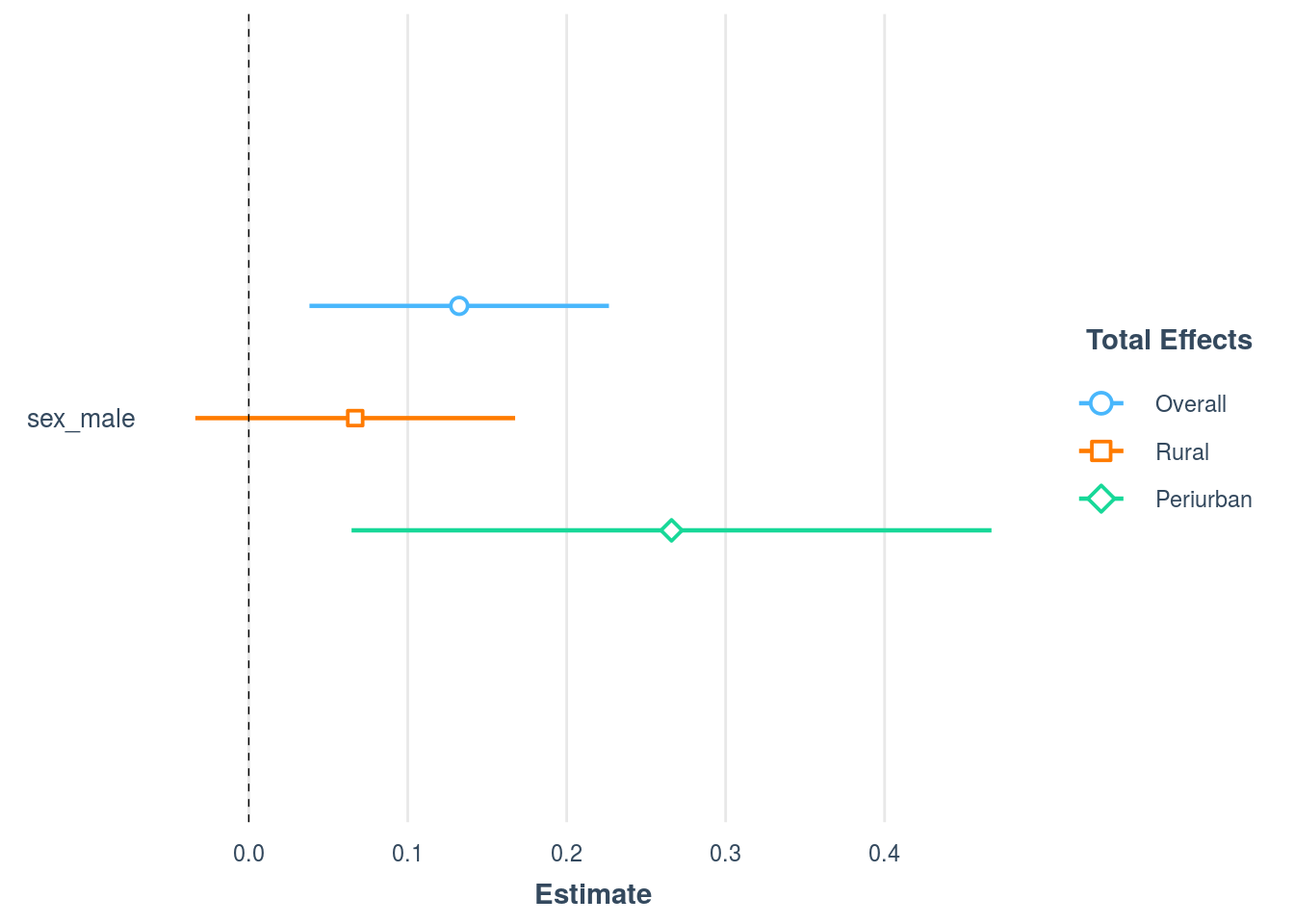
plot_summs(cde, cde_r, cde_u, scale = TRUE, coefs = c("sex_male"), legend.title = "Controlled Direct Effects",
           model.names = c("Overall", "Rural", "Periurban"), robust = T)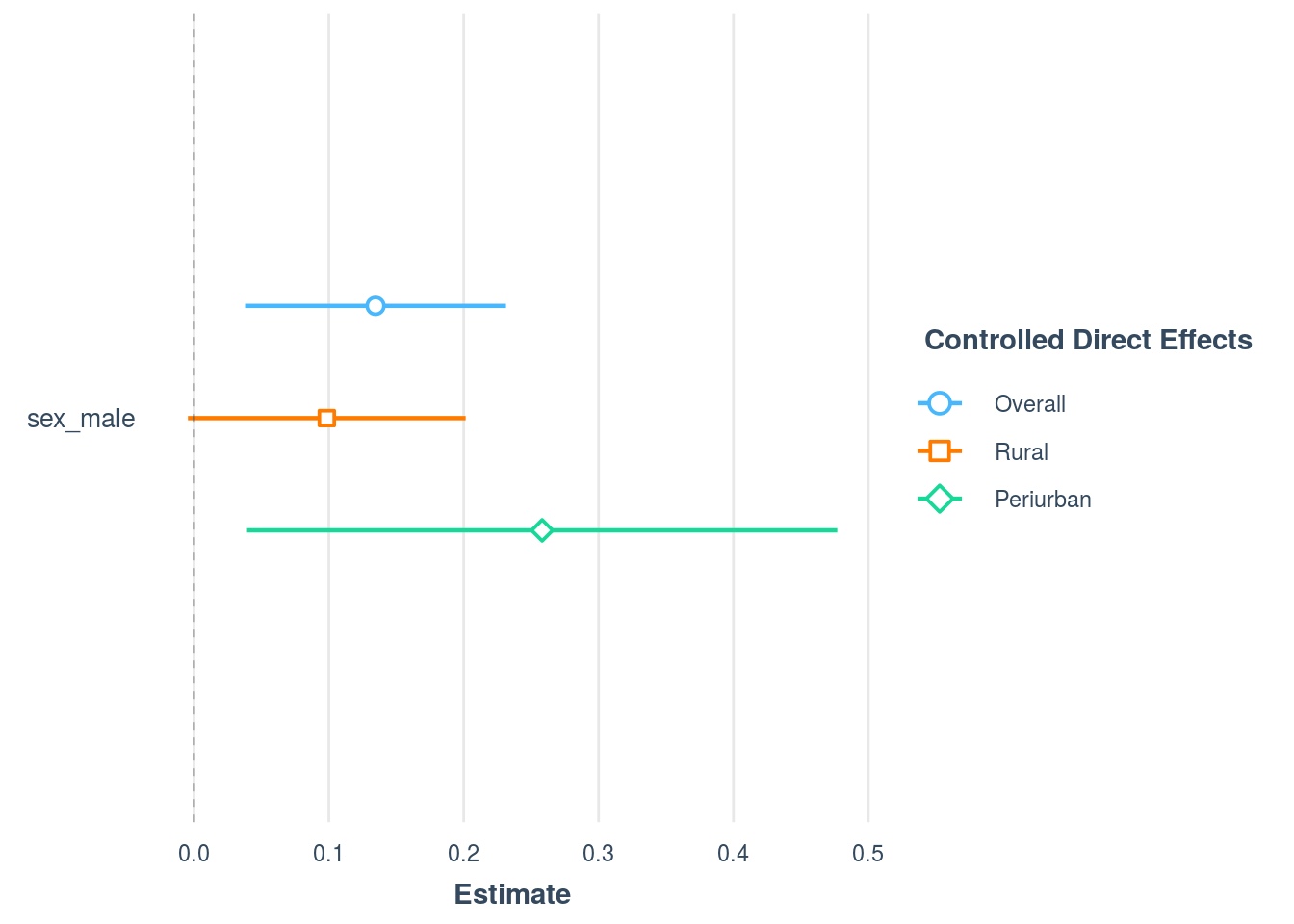
plot_summs(cde, cde_r, cde_u, scale = TRUE, coefs = c("work_out"), legend.title = "Effect of Mediator on Outcome",
           model.names = c("Overall", "Rural", "Periurban"), robust = T)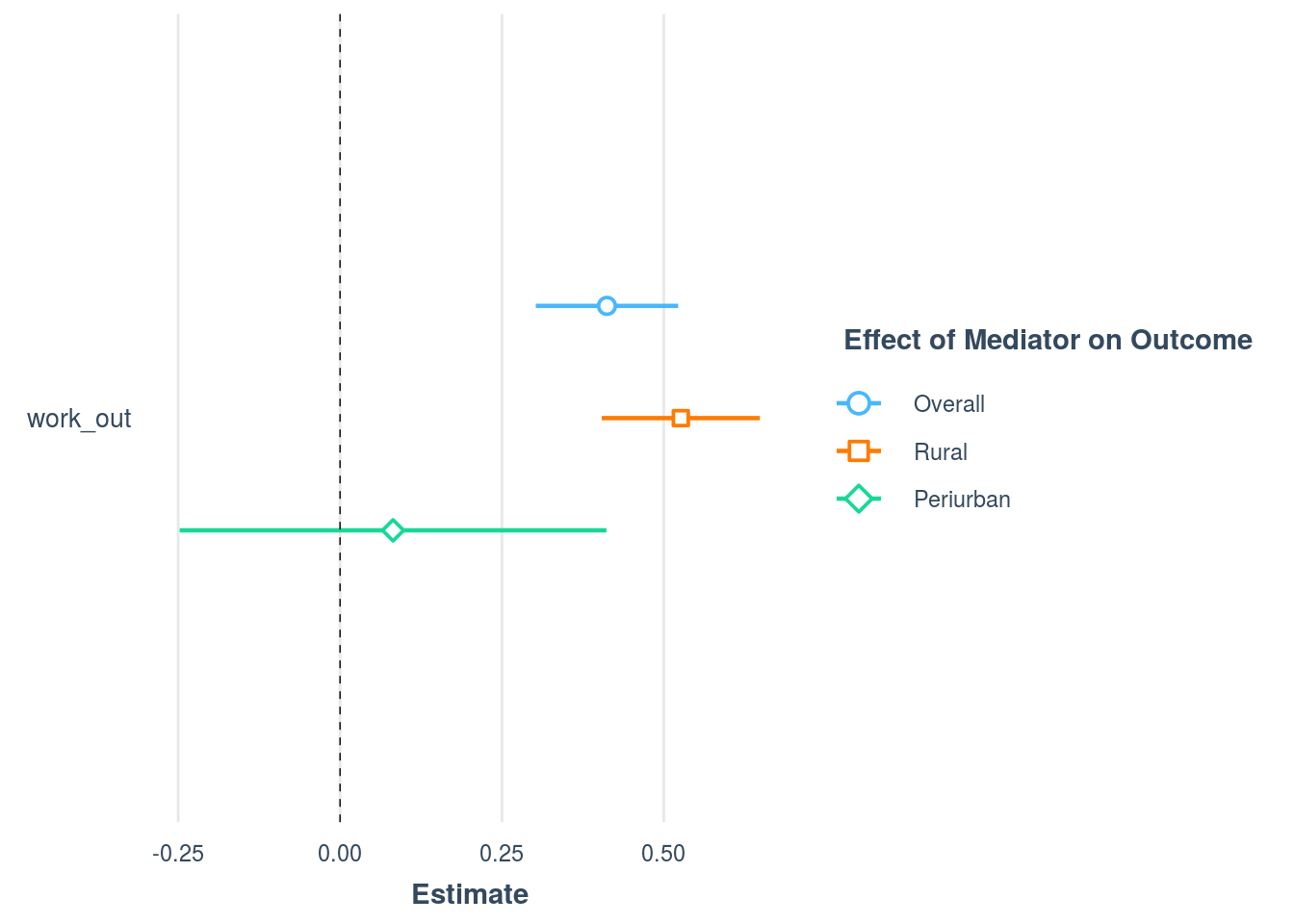
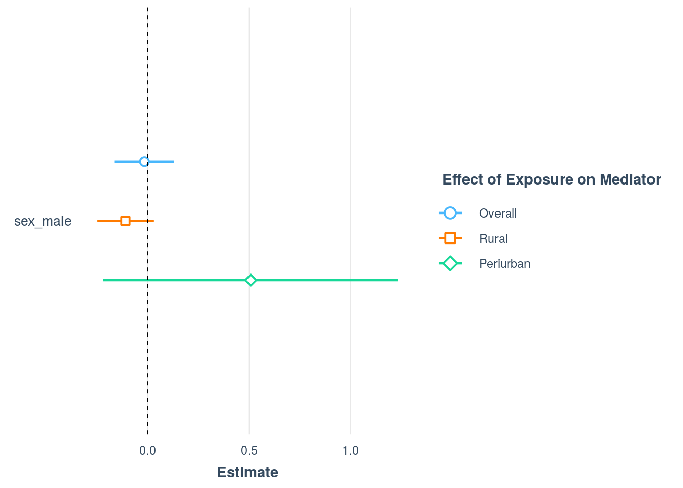
plot_summs(nie, nie_r, nie_u, scale = TRUE, coefs = c("sex_male"), legend.title = "Effect of Exposure on Mediator",
           model.names = c("Overall", "Rural", "Periurban"), robust = T)