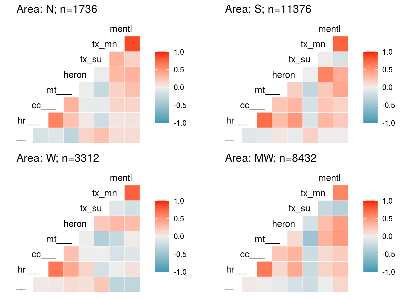
GEGRAPHIC STRATA
NorthEast
# -----------------
# Data
# -----------------
usa.N <- usa.sf %>%
  filter(loc == "N")

nb.map.N <- poly2nb(usa.N)
#nb2INLA("map.graph.N",nb.map.N)

index.N <- usa.N %>%
  dplyr::select(County.Code, ALAND) %>%
  st_set_geometry(NULL) %>%
  mutate(index = 1:nrow(usa.N),
         index2 = index)

dat.N <- data %>%
  inner_join(index.N, by="County.Code") %>%
  inner_join(n.neighbors(nb.map.N), by = "index")

n.N<-nrow(dat.N)

# -----------------
# Formula
# -----------------

N<-c(formula = synthetic_opioid_crude_death_rate ~ 1,
     formula = synthetic_opioid_crude_death_rate ~ 1 +  median_household_income + proportion_homes_no_vehicle + factor(urbanicity) + road_access + urgent_care + population + ALAND + n.neighbors,
     formula = synthetic_opioid_crude_death_rate ~ 1 + f(index, model = "besag", graph = "map.graph.N") + f(year, model = "rw1"),
     formula = synthetic_opioid_crude_death_rate ~ 1 + f(index, model = "besag", graph = "map.graph.N") + f(year, model = "rw1") + median_household_income + proportion_homes_no_vehicle + factor(urbanicity) + road_access + urgent_care + population + ALAND + n.neighbors)

# -----------------
# Model Estimation
# -----------------
names(N)<-c("null", "contextual", "spatial", "full")

INLA:::inla.dynload.workaround()
m.N <- N %>% purrr::map(~inla.batch.safe(formula = ., dat1 = dat.N))

N.s <- m.N %>%
  purrr::map(~Rsq.batch.safe(model = ., dic.null = m.N[[1]]$dic, n = n.N)) %>%
  bind_rows(.id = "formula") %>% mutate(id = row_number())
## [1] 0
## [1] 0.3619135
## [1] 0.9976183
## [1] 0.9976154
# -----------------
# Fixed Effects
# -----------------
m.N[c(2,4)] %>% plot_fixed(
  title = "Overdose",
  filter=10,
  lim = c("median_household_income",  "proportion_homes_no_vehicle", "factor(urbanicity)2", "factor(urbanicity)3", "factor(urbanicity)4", "factor(urbanicity)5", "factor(urbanicity)6", "road_accessTRUE", "urgent_careTRUE", "population", "ALAND", "n.neighbors"),
  breaks=c("1","2"),
  lab_mod=c("contextual","full"), ylab = "exp(mean)", ylim = 2)
##
## Call:
##    c("inla(formula = formula, family = \"poisson\", data = dat1, verbose =
##    F, ", " control.compute = list(config = T, dic = T, cpo = T, waic = T),
##    ", " control.predictor = list(link = 1, compute = TRUE), control.fixed
##    = list(correlation.matrix = T))" )
## Time used:
##     Pre = 4.69, Running = 4.94, Post = 0.752, Total = 10.4
## Fixed effects:
##                               mean    sd 0.025quant 0.5quant 0.975quant   mode
## (Intercept)                  1.467 0.274      0.931    1.467      2.007  1.466
## median_household_income      0.000 0.000      0.000    0.000      0.000  0.000
## proportion_homes_no_vehicle -0.011 0.006     -0.023   -0.011      0.001 -0.011
## factor(urbanicity)2         -0.209 0.141     -0.485   -0.209      0.068 -0.209
## factor(urbanicity)3         -0.261 0.148     -0.553   -0.261      0.030 -0.261
## factor(urbanicity)4         -0.293 0.165     -0.618   -0.294      0.031 -0.294
## factor(urbanicity)5         -0.305 0.160     -0.620   -0.305      0.011 -0.305
## factor(urbanicity)6         -0.453 0.171     -0.788   -0.453     -0.117 -0.454
## road_accessTRUE              0.060 0.090     -0.116    0.060      0.236  0.060
## urgent_careTRUE             -0.242 0.061     -0.363   -0.242     -0.121 -0.242
## population                   0.000 0.000      0.000    0.000      0.000  0.000
## ALAND                        0.000 0.000      0.000    0.000      0.000  0.000
## n.neighbors                  0.006 0.019     -0.031    0.006      0.043  0.006
##                             kld
## (Intercept)                   0
## median_household_income       0
## proportion_homes_no_vehicle   0
## factor(urbanicity)2           0
## factor(urbanicity)3           0
## factor(urbanicity)4           0
## factor(urbanicity)5           0
## factor(urbanicity)6           0
## road_accessTRUE               0
## urgent_careTRUE               0
## population                    0
## ALAND                         0
## n.neighbors                   0
##
## Linear combinations (derived):
##                             ID   mean    sd 0.025quant 0.5quant 0.975quant
## (Intercept)                  1  1.468 0.274      0.931    1.467      2.006
## median_household_income      2  0.000 0.000      0.000    0.000      0.000
## proportion_homes_no_vehicle  3 -0.011 0.006     -0.023   -0.011      0.001
## factor(urbanicity)2          4 -0.209 0.141     -0.485   -0.209      0.068
## factor(urbanicity)3          5 -0.261 0.148     -0.553   -0.261      0.030
## factor(urbanicity)4          6 -0.293 0.165     -0.618   -0.293      0.031
## factor(urbanicity)5          7 -0.305 0.160     -0.619   -0.305      0.011
## factor(urbanicity)6          8 -0.453 0.171     -0.788   -0.453     -0.117
## road_accessTRUE              9  0.060 0.090     -0.116    0.060      0.236
## urgent_careTRUE             10 -0.242 0.061     -0.363   -0.242     -0.121
## population                  11  0.000 0.000      0.000    0.000      0.000
## ALAND                       12  0.000 0.000      0.000    0.000      0.000
## n.neighbors                 13  0.006 0.019     -0.031    0.006      0.043
##                               mode kld
## (Intercept)                  1.467   0
## median_household_income      0.000   0
## proportion_homes_no_vehicle -0.011   0
## factor(urbanicity)2         -0.209   0
## factor(urbanicity)3         -0.261   0
## factor(urbanicity)4         -0.294   0
## factor(urbanicity)5         -0.305   0
## factor(urbanicity)6         -0.453   0
## road_accessTRUE              0.060   0
## urgent_careTRUE             -0.242   0
## population                   0.000   0
## ALAND                        0.000   0
## n.neighbors                  0.006   0
##
## Random effects:
##   Name     Model
##     index Besags ICAR model
##    year RW1 model
##
## Model hyperparameters:
##                     mean    sd 0.025quant 0.5quant 0.975quant mode
## Precision for index 2.29 0.311       1.74     2.26       2.96 2.22
## Precision for year  4.38 2.090       1.45     4.02       9.45 3.27
##
## Expected number of effective parameters(stdev): 167.21(4.97)
## Number of equivalent replicates : 10.38
##
## Deviance Information Criterion (DIC) ...............: 4393.42
## Deviance Information Criterion (DIC, saturated) ....: 1345.88
## Effective number of parameters .....................: 166.84
##
## Watanabe-Akaike information criterion (WAIC) ...: 4441.81
## Effective number of parameters .................: 179.91
##
## Marginal log-Likelihood:  -2588.55
## CPO and PIT are computed
##
## Posterior marginals for the linear predictor and
##  the fitted values are computed
##
## Call:
##    c("inla(formula = formula, family = \"poisson\", data = dat1, verbose =
##    F, ", " control.compute = list(config = T, dic = T, cpo = T, waic = T),
##    ", " control.predictor = list(link = 1, compute = TRUE), control.fixed
##    = list(correlation.matrix = T))" )
## Time used:
##     Pre = 3.13, Running = 3.93, Post = 0.599, Total = 7.66
## Fixed effects:
##              mean    sd 0.025quant 0.5quant 0.975quant  mode kld
## (Intercept) 0.733 0.021      0.692    0.733      0.773 0.733   0
##
## Linear combinations (derived):
##             ID  mean    sd 0.025quant 0.5quant 0.975quant  mode kld
## (Intercept)  1 0.733 0.021      0.693    0.733      0.774 0.733   0
##
## Random effects:
##   Name     Model
##     index Besags ICAR model
##    year RW1 model
##
## Model hyperparameters:
##                     mean    sd 0.025quant 0.5quant 0.975quant mode
## Precision for index 2.02 0.255       1.56     2.00       2.56 1.97
## Precision for year  4.44 2.119       1.47     4.08       9.58 3.31
##
## Expected number of effective parameters(stdev): 168.56(4.63)
## Number of equivalent replicates : 10.30
##
## Deviance Information Criterion (DIC) ...............: 4393.74
## Deviance Information Criterion (DIC, saturated) ....: 1346.20
## Effective number of parameters .....................: 168.09
##
## Watanabe-Akaike information criterion (WAIC) ...: 4442.74
## Effective number of parameters .................: 181.26
##
## Marginal log-Likelihood:  -2482.51
## CPO and PIT are computed
##
## Posterior marginals for the linear predictor and
##  the fitted values are computed
##
## Call:
##    c("inla(formula = formula, family = \"poisson\", data = dat1, verbose =
##    F, ", " control.compute = list(config = T, dic = T, cpo = T, waic = T),
##    ", " control.predictor = list(link = 1, compute = TRUE), control.fixed
##    = list(correlation.matrix = T))" )
## Time used:
##     Pre = 4.69, Running = 4.94, Post = 0.752, Total = 10.4
## Fixed effects:
##                               mean    sd 0.025quant 0.5quant 0.975quant   mode
## (Intercept)                  1.467 0.274      0.931    1.467      2.007  1.466
## median_household_income      0.000 0.000      0.000    0.000      0.000  0.000
## proportion_homes_no_vehicle -0.011 0.006     -0.023   -0.011      0.001 -0.011
## factor(urbanicity)2         -0.209 0.141     -0.485   -0.209      0.068 -0.209
## factor(urbanicity)3         -0.261 0.148     -0.553   -0.261      0.030 -0.261
## factor(urbanicity)4         -0.293 0.165     -0.618   -0.294      0.031 -0.294
## factor(urbanicity)5         -0.305 0.160     -0.620   -0.305      0.011 -0.305
## factor(urbanicity)6         -0.453 0.171     -0.788   -0.453     -0.117 -0.454
## road_accessTRUE              0.060 0.090     -0.116    0.060      0.236  0.060
## urgent_careTRUE             -0.242 0.061     -0.363   -0.242     -0.121 -0.242
## population                   0.000 0.000      0.000    0.000      0.000  0.000
## ALAND                        0.000 0.000      0.000    0.000      0.000  0.000
## n.neighbors                  0.006 0.019     -0.031    0.006      0.043  0.006
##                             kld
## (Intercept)                   0
## median_household_income       0
## proportion_homes_no_vehicle   0
## factor(urbanicity)2           0
## factor(urbanicity)3           0
## factor(urbanicity)4           0
## factor(urbanicity)5           0
## factor(urbanicity)6           0
## road_accessTRUE               0
## urgent_careTRUE               0
## population                    0
## ALAND                         0
## n.neighbors                   0
##
## Linear combinations (derived):
##                             ID   mean    sd 0.025quant 0.5quant 0.975quant
## (Intercept)                  1  1.468 0.274      0.931    1.467      2.006
## median_household_income      2  0.000 0.000      0.000    0.000      0.000
## proportion_homes_no_vehicle  3 -0.011 0.006     -0.023   -0.011      0.001
## factor(urbanicity)2          4 -0.209 0.141     -0.485   -0.209      0.068
## factor(urbanicity)3          5 -0.261 0.148     -0.553   -0.261      0.030
## factor(urbanicity)4          6 -0.293 0.165     -0.618   -0.293      0.031
## factor(urbanicity)5          7 -0.305 0.160     -0.619   -0.305      0.011
## factor(urbanicity)6          8 -0.453 0.171     -0.788   -0.453     -0.117
## road_accessTRUE              9  0.060 0.090     -0.116    0.060      0.236
## urgent_careTRUE             10 -0.242 0.061     -0.363   -0.242     -0.121
## population                  11  0.000 0.000      0.000    0.000      0.000
## ALAND                       12  0.000 0.000      0.000    0.000      0.000
## n.neighbors                 13  0.006 0.019     -0.031    0.006      0.043
##                               mode kld
## (Intercept)                  1.467   0
## median_household_income      0.000   0
## proportion_homes_no_vehicle -0.011   0
## factor(urbanicity)2         -0.209   0
## factor(urbanicity)3         -0.261   0
## factor(urbanicity)4         -0.294   0
## factor(urbanicity)5         -0.305   0
## factor(urbanicity)6         -0.453   0
## road_accessTRUE              0.060   0
## urgent_careTRUE             -0.242   0
## population                   0.000   0
## ALAND                        0.000   0
## n.neighbors                  0.006   0
##
## Random effects:
##   Name     Model
##     index Besags ICAR model
##    year RW1 model
##
## Model hyperparameters:
##                     mean    sd 0.025quant 0.5quant 0.975quant mode
## Precision for index 2.29 0.311       1.74     2.26       2.96 2.22
## Precision for year  4.38 2.090       1.45     4.02       9.45 3.27
##
## Expected number of effective parameters(stdev): 167.21(4.97)
## Number of equivalent replicates : 10.38
##
## Deviance Information Criterion (DIC) ...............: 4393.42
## Deviance Information Criterion (DIC, saturated) ....: 1345.88
## Effective number of parameters .....................: 166.84
##
## Watanabe-Akaike information criterion (WAIC) ...: 4441.81
## Effective number of parameters .................: 179.91
##
## Marginal log-Likelihood:  -2588.55
## CPO and PIT are computed
##
## Posterior marginals for the linear predictor and
##  the fitted values are computed
South
# -----------------
# Data
# -----------------
usa.S <- usa.sf %>%
  filter(loc == "S")

nb.map.S <- poly2nb(usa.S)
#nb2INLA("map.graph.S",nb.map.S)

index.S <- usa.S %>%
  dplyr::select(County.Code, ALAND) %>%
  st_set_geometry(NULL) %>%
  mutate(index = 1:nrow(usa.S),
         index2 = index)

dat.S <- data %>%
  inner_join(index.S, by="County.Code") %>%
  inner_join(n.neighbors(nb.map.S), by = "index")

n.S<-nrow(dat.S)

# -----------------
# Formula
# -----------------
S<-c(formula = synthetic_opioid_crude_death_rate ~ 1,
     formula = synthetic_opioid_crude_death_rate ~ 1 +  median_household_income + proportion_homes_no_vehicle + factor(urbanicity) + road_access + urgent_care + population + ALAND + n.neighbors,
     formula = synthetic_opioid_crude_death_rate ~ 1 + f(index, model = "besag", graph = "map.graph.S") + f(year, model = "rw1"),
     formula = synthetic_opioid_crude_death_rate ~ 1 + f(index, model = "besag", graph = "map.graph.S") + f(year, model = "rw1") + median_household_income + proportion_homes_no_vehicle + factor(urbanicity) + road_access + urgent_care + population + ALAND + n.neighbors)

# -----------------
# Model Estimation
# -----------------
names(S)<-c("null", "contextual", "spatial", "full")

INLA:::inla.dynload.workaround()
m.S <- S %>% purrr::map(~inla.batch.safe(formula = ., dat1 = dat.S))

S.s <- m.S %>%
  purrr::map(~Rsq.batch.safe(model = ., dic.null = m.S[[1]]$dic, n = n.S)) %>%
  bind_rows(.id = "formula") %>% mutate(id = row_number())
## [1] 0
## [1] 0.3240257
## [1] 0.9227073
## [1] 0.92264
# -----------------
# Fixed Effects
# -----------------
m.S[c(2,4)] %>% plot_fixed(
  title = "Overdose",
  filter=10,
  lim = c("median_household_income",  "proportion_homes_no_vehicle", "factor(urbanicity)2", "factor(urbanicity)3", "factor(urbanicity)4", "factor(urbanicity)5", "factor(urbanicity)6", "road_accessTRUE", "urgent_careTRUE", "population", "ALAND", "n.neighbors"),
  breaks=c("1","2"),
  lab_mod=c("contextual","full"), ylab = "exp(mean)", ylim = 2)
##
## Call:
##    c("inla(formula = formula, family = \"poisson\", data = dat1, verbose =
##    F, ", " control.compute = list(config = T, dic = T, cpo = T, waic = T),
##    ", " control.predictor = list(link = 1, compute = TRUE), control.fixed
##    = list(correlation.matrix = T))" )
## Time used:
##     Pre = 5.9, Running = 68.6, Post = 6.42, Total = 80.9
## Fixed effects:
##                               mean    sd 0.025quant 0.5quant 0.975quant   mode
## (Intercept)                  0.625 0.130      0.370    0.625      0.880  0.626
## median_household_income      0.000 0.000      0.000    0.000      0.000  0.000
## proportion_homes_no_vehicle  0.008 0.004      0.001    0.008      0.016  0.009
## factor(urbanicity)2         -0.077 0.081     -0.236   -0.077      0.083 -0.077
## factor(urbanicity)3         -0.085 0.088     -0.257   -0.085      0.087 -0.086
## factor(urbanicity)4         -0.193 0.090     -0.369   -0.193     -0.016 -0.193
## factor(urbanicity)5         -0.185 0.089     -0.360   -0.185     -0.009 -0.185
## factor(urbanicity)6         -0.163 0.089     -0.337   -0.163      0.011 -0.163
## road_accessTRUE             -0.014 0.023     -0.060   -0.014      0.031 -0.014
## urgent_careTRUE             -0.133 0.023     -0.178   -0.133     -0.089 -0.134
## population                   0.000 0.000      0.000    0.000      0.000  0.000
## ALAND                        0.000 0.000      0.000    0.000      0.000  0.000
## n.neighbors                 -0.017 0.007     -0.031   -0.017     -0.003 -0.017
##                             kld
## (Intercept)                   0
## median_household_income       0
## proportion_homes_no_vehicle   0
## factor(urbanicity)2           0
## factor(urbanicity)3           0
## factor(urbanicity)4           0
## factor(urbanicity)5           0
## factor(urbanicity)6           0
## road_accessTRUE               0
## urgent_careTRUE               0
## population                    0
## ALAND                         0
## n.neighbors                   0
##
## Linear combinations (derived):
##                             ID   mean    sd 0.025quant 0.5quant 0.975quant
## (Intercept)                  1  0.625 0.130      0.370    0.625      0.880
## median_household_income      2  0.000 0.000      0.000    0.000      0.000
## proportion_homes_no_vehicle  3  0.008 0.004      0.001    0.008      0.016
## factor(urbanicity)2          4 -0.077 0.081     -0.236   -0.077      0.083
## factor(urbanicity)3          5 -0.085 0.088     -0.257   -0.085      0.087
## factor(urbanicity)4          6 -0.192 0.090     -0.369   -0.192     -0.016
## factor(urbanicity)5          7 -0.185 0.089     -0.360   -0.185     -0.009
## factor(urbanicity)6          8 -0.163 0.089     -0.337   -0.163      0.011
## road_accessTRUE              9 -0.014 0.023     -0.060   -0.014      0.031
## urgent_careTRUE             10 -0.133 0.023     -0.178   -0.133     -0.089
## population                  11  0.000 0.000      0.000    0.000      0.000
## ALAND                       12  0.000 0.000      0.000    0.000      0.000
## n.neighbors                 13 -0.017 0.007     -0.031   -0.017     -0.003
##                               mode kld
## (Intercept)                  0.625   0
## median_household_income      0.000   0
## proportion_homes_no_vehicle  0.008   0
## factor(urbanicity)2         -0.077   0
## factor(urbanicity)3         -0.085   0
## factor(urbanicity)4         -0.192   0
## factor(urbanicity)5         -0.185   0
## factor(urbanicity)6         -0.163   0
## road_accessTRUE             -0.014   0
## urgent_careTRUE             -0.133   0
## population                   0.000   0
## ALAND                        0.000   0
## n.neighbors                 -0.017   0
##
## Random effects:
##   Name     Model
##     index Besags ICAR model
##    year RW1 model
##
## Model hyperparameters:
##                      mean    sd 0.025quant 0.5quant 0.975quant mode
## Precision for index  4.57 0.289       4.02     4.56       5.16 4.54
## Precision for year  12.75 6.066       4.28    11.68      27.49 9.50
##
## Expected number of effective parameters(stdev): 597.71(17.13)
## Number of equivalent replicates : 19.03
##
## Deviance Information Criterion (DIC) ...............: 26467.31
## Deviance Information Criterion (DIC, saturated) ....: 5265.57
## Effective number of parameters .....................: 594.89
##
## Watanabe-Akaike information criterion (WAIC) ...: 26451.22
## Effective number of parameters .................: 502.21
##
## Marginal log-Likelihood:  -14661.75
## CPO and PIT are computed
##
## Posterior marginals for the linear predictor and
##  the fitted values are computed
##
## Call:
##    c("inla(formula = formula, family = \"poisson\", data = dat1, verbose =
##    F, ", " control.compute = list(config = T, dic = T, cpo = T, waic = T),
##    ", " control.predictor = list(link = 1, compute = TRUE), control.fixed
##    = list(correlation.matrix = T))" )
## Time used:
##     Pre = 3.78, Running = 50.1, Post = 4.24, Total = 58.1
## Fixed effects:
##              mean    sd 0.025quant 0.5quant 0.975quant  mode kld
## (Intercept) 0.356 0.009      0.338    0.356      0.374 0.356   0
##
## Linear combinations (derived):
##             ID  mean    sd 0.025quant 0.5quant 0.975quant  mode kld
## (Intercept)  1 0.356 0.009      0.338    0.356      0.374 0.356   0
##
## Random effects:
##   Name     Model
##     index Besags ICAR model
##    year RW1 model
##
## Model hyperparameters:
##                      mean    sd 0.025quant 0.5quant 0.975quant mode
## Precision for index  4.01 0.244       3.56     4.01       4.52 3.99
## Precision for year  12.90 6.089       4.30    11.87      27.66 9.68
##
## Expected number of effective parameters(stdev): 626.74(16.88)
## Number of equivalent replicates : 18.15
##
## Deviance Information Criterion (DIC) ...............: 26515.03
## Deviance Information Criterion (DIC, saturated) ....: 5313.29
## Effective number of parameters .....................: 623.71
##
## Watanabe-Akaike information criterion (WAIC) ...: 26495.54
## Effective number of parameters .................: 522.75
##
## Marginal log-Likelihood:  -14584.59
## CPO and PIT are computed
##
## Posterior marginals for the linear predictor and
##  the fitted values are computed
##
## Call:
##    c("inla(formula = formula, family = \"poisson\", data = dat1, verbose =
##    F, ", " control.compute = list(config = T, dic = T, cpo = T, waic = T),
##    ", " control.predictor = list(link = 1, compute = TRUE), control.fixed
##    = list(correlation.matrix = T))" )
## Time used:
##     Pre = 5.9, Running = 68.6, Post = 6.42, Total = 80.9
## Fixed effects:
##                               mean    sd 0.025quant 0.5quant 0.975quant   mode
## (Intercept)                  0.625 0.130      0.370    0.625      0.880  0.626
## median_household_income      0.000 0.000      0.000    0.000      0.000  0.000
## proportion_homes_no_vehicle  0.008 0.004      0.001    0.008      0.016  0.009
## factor(urbanicity)2         -0.077 0.081     -0.236   -0.077      0.083 -0.077
## factor(urbanicity)3         -0.085 0.088     -0.257   -0.085      0.087 -0.086
## factor(urbanicity)4         -0.193 0.090     -0.369   -0.193     -0.016 -0.193
## factor(urbanicity)5         -0.185 0.089     -0.360   -0.185     -0.009 -0.185
## factor(urbanicity)6         -0.163 0.089     -0.337   -0.163      0.011 -0.163
## road_accessTRUE             -0.014 0.023     -0.060   -0.014      0.031 -0.014
## urgent_careTRUE             -0.133 0.023     -0.178   -0.133     -0.089 -0.134
## population                   0.000 0.000      0.000    0.000      0.000  0.000
## ALAND                        0.000 0.000      0.000    0.000      0.000  0.000
## n.neighbors                 -0.017 0.007     -0.031   -0.017     -0.003 -0.017
##                             kld
## (Intercept)                   0
## median_household_income       0
## proportion_homes_no_vehicle   0
## factor(urbanicity)2           0
## factor(urbanicity)3           0
## factor(urbanicity)4           0
## factor(urbanicity)5           0
## factor(urbanicity)6           0
## road_accessTRUE               0
## urgent_careTRUE               0
## population                    0
## ALAND                         0
## n.neighbors                   0
##
## Linear combinations (derived):
##                             ID   mean    sd 0.025quant 0.5quant 0.975quant
## (Intercept)                  1  0.625 0.130      0.370    0.625      0.880
## median_household_income      2  0.000 0.000      0.000    0.000      0.000
## proportion_homes_no_vehicle  3  0.008 0.004      0.001    0.008      0.016
## factor(urbanicity)2          4 -0.077 0.081     -0.236   -0.077      0.083
## factor(urbanicity)3          5 -0.085 0.088     -0.257   -0.085      0.087
## factor(urbanicity)4          6 -0.192 0.090     -0.369   -0.192     -0.016
## factor(urbanicity)5          7 -0.185 0.089     -0.360   -0.185     -0.009
## factor(urbanicity)6          8 -0.163 0.089     -0.337   -0.163      0.011
## road_accessTRUE              9 -0.014 0.023     -0.060   -0.014      0.031
## urgent_careTRUE             10 -0.133 0.023     -0.178   -0.133     -0.089
## population                  11  0.000 0.000      0.000    0.000      0.000
## ALAND                       12  0.000 0.000      0.000    0.000      0.000
## n.neighbors                 13 -0.017 0.007     -0.031   -0.017     -0.003
##                               mode kld
## (Intercept)                  0.625   0
## median_household_income      0.000   0
## proportion_homes_no_vehicle  0.008   0
## factor(urbanicity)2         -0.077   0
## factor(urbanicity)3         -0.085   0
## factor(urbanicity)4         -0.192   0
## factor(urbanicity)5         -0.185   0
## factor(urbanicity)6         -0.163   0
## road_accessTRUE             -0.014   0
## urgent_careTRUE             -0.133   0
## population                   0.000   0
## ALAND                        0.000   0
## n.neighbors                 -0.017   0
##
## Random effects:
##   Name     Model
##     index Besags ICAR model
##    year RW1 model
##
## Model hyperparameters:
##                      mean    sd 0.025quant 0.5quant 0.975quant mode
## Precision for index  4.57 0.289       4.02     4.56       5.16 4.54
## Precision for year  12.75 6.066       4.28    11.68      27.49 9.50
##
## Expected number of effective parameters(stdev): 597.71(17.13)
## Number of equivalent replicates : 19.03
##
## Deviance Information Criterion (DIC) ...............: 26467.31
## Deviance Information Criterion (DIC, saturated) ....: 5265.57
## Effective number of parameters .....................: 594.89
##
## Watanabe-Akaike information criterion (WAIC) ...: 26451.22
## Effective number of parameters .................: 502.21
##
## Marginal log-Likelihood:  -14661.75
## CPO and PIT are computed
##
## Posterior marginals for the linear predictor and
##  the fitted values are computed
West
# -----------------
# Data
# -----------------
usa.W <- usa.sf %>%
  filter(loc == "W")

nb.map.W <- poly2nb(usa.W)
#nb2INLA("map.graph.W",nb.map.W)

index.W <- usa.W %>%
  dplyr::select(County.Code, ALAND) %>%
  st_set_geometry(NULL) %>%
  mutate(index = 1:nrow(usa.W),
         index2 = index)

dat.W <- data %>%
  inner_join(index.W, by="County.Code") %>%
  inner_join(n.neighbors(nb.map.W), by = "index")

n.W<-nrow(dat.W)

# -----------------
# Formula
# -----------------
W<-c(formula = synthetic_opioid_crude_death_rate ~ 1,
     formula = synthetic_opioid_crude_death_rate ~ 1 +  median_household_income + proportion_homes_no_vehicle + factor(urbanicity) + road_access + urgent_care + urgent_care + population + ALAND + n.neighbors,
     formula = synthetic_opioid_crude_death_rate ~ 1 + f(index, model = "besag", graph = "map.graph.W") + f(year, model = "rw1"),
     formula = synthetic_opioid_crude_death_rate ~ 1 + f(index, model = "besag", graph = "map.graph.W") + f(year, model = "rw1") + median_household_income + proportion_homes_no_vehicle + factor(urbanicity) + road_access + urgent_care + urgent_care + population + ALAND + n.neighbors)

# -----------------
# Model Estimation
# -----------------
names(W)<-c("null", "contextual", "spatial", "full")

INLA:::inla.dynload.workaround()
m.W <- W %>% purrr::map(~inla.batch.safe(formula = ., dat1 = dat.W))

W.s <- m.W %>%
  purrr::map(~Rsq.batch.safe(model = ., dic.null = m.W[[1]]$dic, n = n.W)) %>%
  bind_rows(.id = "formula") %>% mutate(id = row_number())
## [1] 0
## [1] 0.009904794
## [1] 0.2093016
## [1] 0.2106695
# -----------------
# Fixed Effects
# -----------------
m.W[c(2,4)] %>% plot_fixed(
  title = "Overdose",
  filter=10,
  lim = c("median_household_income",  "proportion_homes_no_vehicle", "factor(urbanicity)2", "factor(urbanicity)3", "factor(urbanicity)4", "factor(urbanicity)5", "factor(urbanicity)6", "road_accessTRUE", "urgent_careTRUE", "population", "ALAND", "n.neighbors"),
  breaks=c("1","2"),
  lab_mod=c("contextual","full"), ylab = "exp(mean)", ylim = 2)
##
## Call:
##    c("inla(formula = formula, family = \"poisson\", data = dat1, verbose =
##    F, ", " control.compute = list(config = T, dic = T, cpo = T, waic = T),
##    ", " control.predictor = list(link = 1, compute = TRUE), control.fixed
##    = list(correlation.matrix = T))" )
## Time used:
##     Pre = 6.16, Running = 11, Post = 1.23, Total = 18.4
## Fixed effects:
##                               mean    sd 0.025quant 0.5quant 0.975quant   mode
## (Intercept)                  0.186 0.248     -0.301    0.186      0.671  0.187
## median_household_income      0.000 0.000      0.000    0.000      0.000  0.000
## proportion_homes_no_vehicle  0.003 0.009     -0.014    0.003      0.020  0.003
## factor(urbanicity)2         -0.247 0.166     -0.572   -0.247      0.080 -0.248
## factor(urbanicity)3         -0.145 0.162     -0.462   -0.146      0.174 -0.147
## factor(urbanicity)4         -0.290 0.173     -0.628   -0.290      0.050 -0.290
## factor(urbanicity)5         -0.267 0.170     -0.601   -0.267      0.067 -0.268
## factor(urbanicity)6         -0.272 0.175     -0.615   -0.272      0.072 -0.273
## road_accessTRUE             -0.040 0.045     -0.130   -0.041      0.049 -0.041
## urgent_careTRUE             -0.036 0.048     -0.130   -0.036      0.058 -0.036
## population                   0.000 0.000      0.000    0.000      0.000  0.000
## ALAND                        0.000 0.000      0.000    0.000      0.000  0.000
## n.neighbors                  0.017 0.013     -0.009    0.017      0.042  0.017
##                             kld
## (Intercept)                   0
## median_household_income       0
## proportion_homes_no_vehicle   0
## factor(urbanicity)2           0
## factor(urbanicity)3           0
## factor(urbanicity)4           0
## factor(urbanicity)5           0
## factor(urbanicity)6           0
## road_accessTRUE               0
## urgent_careTRUE               0
## population                    0
## ALAND                         0
## n.neighbors                   0
##
## Linear combinations (derived):
##                             ID   mean    sd 0.025quant 0.5quant 0.975quant
## (Intercept)                  1  0.186 0.247     -0.301    0.186      0.671
## median_household_income      2  0.000 0.000      0.000    0.000      0.000
## proportion_homes_no_vehicle  3  0.003 0.009     -0.014    0.003      0.020
## factor(urbanicity)2          4 -0.247 0.166     -0.572   -0.247      0.079
## factor(urbanicity)3          5 -0.145 0.162     -0.463   -0.145      0.173
## factor(urbanicity)4          6 -0.289 0.173     -0.628   -0.290      0.049
## factor(urbanicity)5          7 -0.267 0.170     -0.601   -0.267      0.067
## factor(urbanicity)6          8 -0.272 0.175     -0.615   -0.272      0.072
## road_accessTRUE              9 -0.041 0.045     -0.130   -0.041      0.049
## urgent_careTRUE             10 -0.036 0.048     -0.130   -0.036      0.058
## population                  11  0.000 0.000      0.000    0.000      0.000
## ALAND                       12  0.000 0.000      0.000    0.000      0.000
## n.neighbors                 13  0.017 0.013     -0.009    0.017      0.043
##                               mode kld
## (Intercept)                  0.186   0
## median_household_income      0.000   0
## proportion_homes_no_vehicle  0.003   0
## factor(urbanicity)2         -0.247   0
## factor(urbanicity)3         -0.146   0
## factor(urbanicity)4         -0.290   0
## factor(urbanicity)5         -0.267   0
## factor(urbanicity)6         -0.272   0
## road_accessTRUE             -0.041   0
## urgent_careTRUE             -0.036   0
## population                   0.000   0
## ALAND                        0.000   0
## n.neighbors                  0.017   0
##
## Random effects:
##   Name     Model
##     index Besags ICAR model
##    year RW1 model
##
## Model hyperparameters:
##                      mean   sd 0.025quant 0.5quant 0.975quant mode
## Precision for index  8.86 1.48       6.35     8.73      12.11 8.47
## Precision for year  13.68 7.47       4.02    12.14      32.54 9.25
##
## Expected number of effective parameters(stdev): 99.06(8.95)
## Number of equivalent replicates : 33.43
##
## Deviance Information Criterion (DIC) ...............: 6788.60
## Deviance Information Criterion (DIC, saturated) ....: 1142.00
## Effective number of parameters .....................: 99.12
##
## Watanabe-Akaike information criterion (WAIC) ...: 6714.88
## Effective number of parameters .................: 24.54
##
## Marginal log-Likelihood:  -3861.26
## CPO and PIT are computed
##
## Posterior marginals for the linear predictor and
##  the fitted values are computed
##
## Call:
##    c("inla(formula = formula, family = \"poisson\", data = dat1, verbose =
##    F, ", " control.compute = list(config = T, dic = T, cpo = T, waic = T),
##    ", " control.predictor = list(link = 1, compute = TRUE), control.fixed
##    = list(correlation.matrix = T))" )
## Time used:
##     Pre = 4.12, Running = 8.55, Post = 1.08, Total = 13.8
## Fixed effects:
##               mean    sd 0.025quant 0.5quant 0.975quant   mode kld
## (Intercept) -0.022 0.018     -0.058   -0.022      0.014 -0.022   0
##
## Linear combinations (derived):
##             ID   mean    sd 0.025quant 0.5quant 0.975quant   mode kld
## (Intercept)  1 -0.022 0.018     -0.058   -0.022      0.014 -0.022   0
##
## Random effects:
##   Name     Model
##     index Besags ICAR model
##    year RW1 model
##
## Model hyperparameters:
##                      mean   sd 0.025quant 0.5quant 0.975quant mode
## Precision for index  8.71 1.41       6.28     8.59      11.80 8.36
## Precision for year  13.65 7.50       4.03    12.08      32.59 9.19
##
## Expected number of effective parameters(stdev): 90.88(9.04)
## Number of equivalent replicates : 36.44
##
## Deviance Information Criterion (DIC) ...............: 6778.34
## Deviance Information Criterion (DIC, saturated) ....: 1131.73
## Effective number of parameters .....................: 91.12
##
## Watanabe-Akaike information criterion (WAIC) ...: 6710.18
## Effective number of parameters .................: 22.27
##
## Marginal log-Likelihood:  -3740.79
## CPO and PIT are computed
##
## Posterior marginals for the linear predictor and
##  the fitted values are computed
##
## Call:
##    c("inla(formula = formula, family = \"poisson\", data = dat1, verbose =
##    F, ", " control.compute = list(config = T, dic = T, cpo = T, waic = T),
##    ", " control.predictor = list(link = 1, compute = TRUE), control.fixed
##    = list(correlation.matrix = T))" )
## Time used:
##     Pre = 6.16, Running = 11, Post = 1.23, Total = 18.4
## Fixed effects:
##                               mean    sd 0.025quant 0.5quant 0.975quant   mode
## (Intercept)                  0.186 0.248     -0.301    0.186      0.671  0.187
## median_household_income      0.000 0.000      0.000    0.000      0.000  0.000
## proportion_homes_no_vehicle  0.003 0.009     -0.014    0.003      0.020  0.003
## factor(urbanicity)2         -0.247 0.166     -0.572   -0.247      0.080 -0.248
## factor(urbanicity)3         -0.145 0.162     -0.462   -0.146      0.174 -0.147
## factor(urbanicity)4         -0.290 0.173     -0.628   -0.290      0.050 -0.290
## factor(urbanicity)5         -0.267 0.170     -0.601   -0.267      0.067 -0.268
## factor(urbanicity)6         -0.272 0.175     -0.615   -0.272      0.072 -0.273
## road_accessTRUE             -0.040 0.045     -0.130   -0.041      0.049 -0.041
## urgent_careTRUE             -0.036 0.048     -0.130   -0.036      0.058 -0.036
## population                   0.000 0.000      0.000    0.000      0.000  0.000
## ALAND                        0.000 0.000      0.000    0.000      0.000  0.000
## n.neighbors                  0.017 0.013     -0.009    0.017      0.042  0.017
##                             kld
## (Intercept)                   0
## median_household_income       0
## proportion_homes_no_vehicle   0
## factor(urbanicity)2           0
## factor(urbanicity)3           0
## factor(urbanicity)4           0
## factor(urbanicity)5           0
## factor(urbanicity)6           0
## road_accessTRUE               0
## urgent_careTRUE               0
## population                    0
## ALAND                         0
## n.neighbors                   0
##
## Linear combinations (derived):
##                             ID   mean    sd 0.025quant 0.5quant 0.975quant
## (Intercept)                  1  0.186 0.247     -0.301    0.186      0.671
## median_household_income      2  0.000 0.000      0.000    0.000      0.000
## proportion_homes_no_vehicle  3  0.003 0.009     -0.014    0.003      0.020
## factor(urbanicity)2          4 -0.247 0.166     -0.572   -0.247      0.079
## factor(urbanicity)3          5 -0.145 0.162     -0.463   -0.145      0.173
## factor(urbanicity)4          6 -0.289 0.173     -0.628   -0.290      0.049
## factor(urbanicity)5          7 -0.267 0.170     -0.601   -0.267      0.067
## factor(urbanicity)6          8 -0.272 0.175     -0.615   -0.272      0.072
## road_accessTRUE              9 -0.041 0.045     -0.130   -0.041      0.049
## urgent_careTRUE             10 -0.036 0.048     -0.130   -0.036      0.058
## population                  11  0.000 0.000      0.000    0.000      0.000
## ALAND                       12  0.000 0.000      0.000    0.000      0.000
## n.neighbors                 13  0.017 0.013     -0.009    0.017      0.043
##                               mode kld
## (Intercept)                  0.186   0
## median_household_income      0.000   0
## proportion_homes_no_vehicle  0.003   0
## factor(urbanicity)2         -0.247   0
## factor(urbanicity)3         -0.146   0
## factor(urbanicity)4         -0.290   0
## factor(urbanicity)5         -0.267   0
## factor(urbanicity)6         -0.272   0
## road_accessTRUE             -0.041   0
## urgent_careTRUE             -0.036   0
## population                   0.000   0
## ALAND                        0.000   0
## n.neighbors                  0.017   0
##
## Random effects:
##   Name     Model
##     index Besags ICAR model
##    year RW1 model
##
## Model hyperparameters:
##                      mean   sd 0.025quant 0.5quant 0.975quant mode
## Precision for index  8.86 1.48       6.35     8.73      12.11 8.47
## Precision for year  13.68 7.47       4.02    12.14      32.54 9.25
##
## Expected number of effective parameters(stdev): 99.06(8.95)
## Number of equivalent replicates : 33.43
##
## Deviance Information Criterion (DIC) ...............: 6788.60
## Deviance Information Criterion (DIC, saturated) ....: 1142.00
## Effective number of parameters .....................: 99.12
##
## Watanabe-Akaike information criterion (WAIC) ...: 6714.88
## Effective number of parameters .................: 24.54
##
## Marginal log-Likelihood:  -3861.26
## CPO and PIT are computed
##
## Posterior marginals for the linear predictor and
##  the fitted values are computed
MidWest
# -----------------
# Data
# -----------------
usa.M <- usa.sf %>%
  filter(loc == "MW")

nb.map.M <- poly2nb(usa.M)
#nb2INLA("map.graph.M",nb.map.M)

index.M <- usa.M %>%
  dplyr::select(County.Code, ALAND) %>%
  st_set_geometry(NULL) %>%
  mutate(index = 1:nrow(usa.M),
         index2 = index)

dat.M <- data %>%
  inner_join(index.M, by="County.Code") %>%
  inner_join(n.neighbors(nb.map.M), by = "index")

n.M<-nrow(dat.M)

# -----------------
# Formula
# -----------------

M<-c(formula = synthetic_opioid_crude_death_rate ~ 1,
     formula = synthetic_opioid_crude_death_rate ~ 1 +  median_household_income + proportion_homes_no_vehicle + factor(urbanicity) + road_access + urgent_care + urgent_care + population + ALAND + n.neighbors,
     formula = synthetic_opioid_crude_death_rate ~ 1 + f(index, model = "besag", graph = "map.graph.M") + f(year, model = "rw1"),
     formula = synthetic_opioid_crude_death_rate ~ 1 + f(index, model = "besag", graph = "map.graph.M") + f(year, model = "rw1") + median_household_income + proportion_homes_no_vehicle + factor(urbanicity) + road_access + urgent_care + urgent_care + population + ALAND + n.neighbors)

# -----------------
# Model Estimation
# -----------------
names(M)<-c("null", "contextual", "spatial", "full")

INLA:::inla.dynload.workaround()
m.M <- M %>% purrr::map(~inla.batch.safe(formula = ., dat1 = dat.M))

M.s <- m.M %>%
  purrr::map(~Rsq.batch.safe(model = ., dic.null = m.M[[1]]$dic, n = n.M)) %>%
  bind_rows(.id = "formula") %>% mutate(id = row_number())
## [1] 0
## [1] 0.4238818
## [1] 0.9138479
## [1] 0.9138585
# -----------------
# Fixed Effects
# -----------------
m.M[c(2,4)] %>% plot_fixed(
  title = "Overdose",
  filter=10,
  lim = c("median_household_income",  "proportion_homes_no_vehicle", "factor(urbanicity)2", "factor(urbanicity)3", "factor(urbanicity)4", "factor(urbanicity)5", "factor(urbanicity)6", "road_accessTRUE", "urgent_careTRUE", "population", "ALAND", "n.neighbors"),
  breaks=c("1","2"),
  lab_mod=c("contextual","full"), ylab = "exp(mean)", ylim = 2)
##
## Call:
##    c("inla(formula = formula, family = \"poisson\", data = dat1, verbose =
##    F, ", " control.compute = list(config = T, dic = T, cpo = T, waic = T),
##    ", " control.predictor = list(link = 1, compute = TRUE), control.fixed
##    = list(correlation.matrix = T))" )
## Time used:
##     Pre = 6.3, Running = 39.9, Post = 3.65, Total = 49.8
## Fixed effects:
##                               mean    sd 0.025quant 0.5quant 0.975quant   mode
## (Intercept)                  0.537 0.171      0.201    0.537      0.872  0.538
## median_household_income      0.000 0.000      0.000    0.000      0.000  0.000
## proportion_homes_no_vehicle  0.017 0.005      0.007    0.018      0.028  0.018
## factor(urbanicity)2         -0.138 0.112     -0.357   -0.138      0.082 -0.138
## factor(urbanicity)3         -0.095 0.116     -0.322   -0.095      0.134 -0.095
## factor(urbanicity)4         -0.177 0.116     -0.404   -0.177      0.051 -0.177
## factor(urbanicity)5         -0.257 0.115     -0.482   -0.257     -0.030 -0.257
## factor(urbanicity)6         -0.254 0.116     -0.482   -0.254     -0.026 -0.255
## road_accessTRUE             -0.019 0.030     -0.077   -0.019      0.039 -0.019
## urgent_careTRUE             -0.073 0.029     -0.131   -0.073     -0.016 -0.073
## population                   0.000 0.000      0.000    0.000      0.000  0.000
## ALAND                        0.000 0.000      0.000    0.000      0.000  0.000
## n.neighbors                  0.003 0.011     -0.018    0.003      0.024  0.003
##                             kld
## (Intercept)                   0
## median_household_income       0
## proportion_homes_no_vehicle   0
## factor(urbanicity)2           0
## factor(urbanicity)3           0
## factor(urbanicity)4           0
## factor(urbanicity)5           0
## factor(urbanicity)6           0
## road_accessTRUE               0
## urgent_careTRUE               0
## population                    0
## ALAND                         0
## n.neighbors                   0
##
## Linear combinations (derived):
##                             ID   mean    sd 0.025quant 0.5quant 0.975quant
## (Intercept)                  1  0.537 0.171      0.201    0.537      0.872
## median_household_income      2  0.000 0.000      0.000    0.000      0.000
## proportion_homes_no_vehicle  3  0.017 0.005      0.007    0.017      0.028
## factor(urbanicity)2          4 -0.137 0.112     -0.357   -0.137      0.081
## factor(urbanicity)3          5 -0.094 0.116     -0.323   -0.094      0.134
## factor(urbanicity)4          6 -0.177 0.116     -0.404   -0.177      0.051
## factor(urbanicity)5          7 -0.256 0.115     -0.482   -0.256     -0.031
## factor(urbanicity)6          8 -0.254 0.116     -0.482   -0.254     -0.026
## road_accessTRUE              9 -0.019 0.030     -0.077   -0.019      0.039
## urgent_careTRUE             10 -0.073 0.029     -0.130   -0.073     -0.016
## population                  11  0.000 0.000      0.000    0.000      0.000
## ALAND                       12  0.000 0.000      0.000    0.000      0.000
## n.neighbors                 13  0.003 0.011     -0.018    0.003      0.024
##                               mode kld
## (Intercept)                  0.538   0
## median_household_income      0.000   0
## proportion_homes_no_vehicle  0.017   0
## factor(urbanicity)2         -0.137   0
## factor(urbanicity)3         -0.094   0
## factor(urbanicity)4         -0.177   0
## factor(urbanicity)5         -0.256   0
## factor(urbanicity)6         -0.254   0
## road_accessTRUE             -0.019   0
## urgent_careTRUE             -0.073   0
## population                   0.000   0
## ALAND                        0.000   0
## n.neighbors                  0.003   0
##
## Random effects:
##   Name     Model
##     index Besags ICAR model
##    year RW1 model
##
## Model hyperparameters:
##                     mean    sd 0.025quant 0.5quant 0.975quant mode
## Precision for index 4.38 0.335       3.76     4.36       5.07 4.34
## Precision for year  8.28 3.942       2.76     7.60      17.86 6.18
##
## Expected number of effective parameters(stdev): 397.87(14.96)
## Number of equivalent replicates : 21.19
##
## Deviance Information Criterion (DIC) ...............: 19579.09
## Deviance Information Criterion (DIC, saturated) ....: 4935.21
## Effective number of parameters .....................: 395.87
##
## Watanabe-Akaike information criterion (WAIC) ...: 19686.51
## Effective number of parameters .................: 430.42
##
## Marginal log-Likelihood:  -10878.80
## CPO and PIT are computed
##
## Posterior marginals for the linear predictor and
##  the fitted values are computed
##
## Call:
##    c("inla(formula = formula, family = \"poisson\", data = dat1, verbose =
##    F, ", " control.compute = list(config = T, dic = T, cpo = T, waic = T),
##    ", " control.predictor = list(link = 1, compute = TRUE), control.fixed
##    = list(correlation.matrix = T))" )
## Time used:
##     Pre = 4.31, Running = 29.9, Post = 3.04, Total = 37.3
## Fixed effects:
##              mean    sd 0.025quant 0.5quant 0.975quant  mode kld
## (Intercept) 0.046 0.012      0.022    0.046       0.07 0.046   0
##
## Linear combinations (derived):
##             ID  mean    sd 0.025quant 0.5quant 0.975quant  mode kld
## (Intercept)  1 0.046 0.012      0.022    0.046       0.07 0.046   0
##
## Random effects:
##   Name     Model
##     index Besags ICAR model
##    year RW1 model
##
## Model hyperparameters:
##                     mean    sd 0.025quant 0.5quant 0.975quant mode
## Precision for index 3.77 0.273       3.26     3.76       4.34 3.74
## Precision for year  8.48 4.034       2.82     7.79      18.28 6.34
##
## Expected number of effective parameters(stdev): 421.40(14.75)
## Number of equivalent replicates : 20.01
##
## Deviance Information Criterion (DIC) ...............: 19626.48
## Deviance Information Criterion (DIC, saturated) ....: 4982.61
## Effective number of parameters .....................: 419.05
##
## Watanabe-Akaike information criterion (WAIC) ...: 19734.47
## Effective number of parameters .................: 449.59
##
## Marginal log-Likelihood:  -10798.26
## CPO and PIT are computed
##
## Posterior marginals for the linear predictor and
##  the fitted values are computed
##
## Call:
##    c("inla(formula = formula, family = \"poisson\", data = dat1, verbose =
##    F, ", " control.compute = list(config = T, dic = T, cpo = T, waic = T),
##    ", " control.predictor = list(link = 1, compute = TRUE), control.fixed
##    = list(correlation.matrix = T))" )
## Time used:
##     Pre = 6.3, Running = 39.9, Post = 3.65, Total = 49.8
## Fixed effects:
##                               mean    sd 0.025quant 0.5quant 0.975quant   mode
## (Intercept)                  0.537 0.171      0.201    0.537      0.872  0.538
## median_household_income      0.000 0.000      0.000    0.000      0.000  0.000
## proportion_homes_no_vehicle  0.017 0.005      0.007    0.018      0.028  0.018
## factor(urbanicity)2         -0.138 0.112     -0.357   -0.138      0.082 -0.138
## factor(urbanicity)3         -0.095 0.116     -0.322   -0.095      0.134 -0.095
## factor(urbanicity)4         -0.177 0.116     -0.404   -0.177      0.051 -0.177
## factor(urbanicity)5         -0.257 0.115     -0.482   -0.257     -0.030 -0.257
## factor(urbanicity)6         -0.254 0.116     -0.482   -0.254     -0.026 -0.255
## road_accessTRUE             -0.019 0.030     -0.077   -0.019      0.039 -0.019
## urgent_careTRUE             -0.073 0.029     -0.131   -0.073     -0.016 -0.073
## population                   0.000 0.000      0.000    0.000      0.000  0.000
## ALAND                        0.000 0.000      0.000    0.000      0.000  0.000
## n.neighbors                  0.003 0.011     -0.018    0.003      0.024  0.003
##                             kld
## (Intercept)                   0
## median_household_income       0
## proportion_homes_no_vehicle   0
## factor(urbanicity)2           0
## factor(urbanicity)3           0
## factor(urbanicity)4           0
## factor(urbanicity)5           0
## factor(urbanicity)6           0
## road_accessTRUE               0
## urgent_careTRUE               0
## population                    0
## ALAND                         0
## n.neighbors                   0
##
## Linear combinations (derived):
##                             ID   mean    sd 0.025quant 0.5quant 0.975quant
## (Intercept)                  1  0.537 0.171      0.201    0.537      0.872
## median_household_income      2  0.000 0.000      0.000    0.000      0.000
## proportion_homes_no_vehicle  3  0.017 0.005      0.007    0.017      0.028
## factor(urbanicity)2          4 -0.137 0.112     -0.357   -0.137      0.081
## factor(urbanicity)3          5 -0.094 0.116     -0.323   -0.094      0.134
## factor(urbanicity)4          6 -0.177 0.116     -0.404   -0.177      0.051
## factor(urbanicity)5          7 -0.256 0.115     -0.482   -0.256     -0.031
## factor(urbanicity)6          8 -0.254 0.116     -0.482   -0.254     -0.026
## road_accessTRUE              9 -0.019 0.030     -0.077   -0.019      0.039
## urgent_careTRUE             10 -0.073 0.029     -0.130   -0.073     -0.016
## population                  11  0.000 0.000      0.000    0.000      0.000
## ALAND                       12  0.000 0.000      0.000    0.000      0.000
## n.neighbors                 13  0.003 0.011     -0.018    0.003      0.024
##                               mode kld
## (Intercept)                  0.538   0
## median_household_income      0.000   0
## proportion_homes_no_vehicle  0.017   0
## factor(urbanicity)2         -0.137   0
## factor(urbanicity)3         -0.094   0
## factor(urbanicity)4         -0.177   0
## factor(urbanicity)5         -0.256   0
## factor(urbanicity)6         -0.254   0
## road_accessTRUE             -0.019   0
## urgent_careTRUE             -0.073   0
## population                   0.000   0
## ALAND                        0.000   0
## n.neighbors                  0.003   0
##
## Random effects:
##   Name     Model
##     index Besags ICAR model
##    year RW1 model
##
## Model hyperparameters:
##                     mean    sd 0.025quant 0.5quant 0.975quant mode
## Precision for index 4.38 0.335       3.76     4.36       5.07 4.34
## Precision for year  8.28 3.942       2.76     7.60      17.86 6.18
##
## Expected number of effective parameters(stdev): 397.87(14.96)
## Number of equivalent replicates : 21.19
##
## Deviance Information Criterion (DIC) ...............: 19579.09
## Deviance Information Criterion (DIC, saturated) ....: 4935.21
## Effective number of parameters .....................: 395.87
##
## Watanabe-Akaike information criterion (WAIC) ...: 19686.51
## Effective number of parameters .................: 430.42
##
## Marginal log-Likelihood:  -10878.80
## CPO and PIT are computed
##
## Posterior marginals for the linear predictor and
##  the fitted values are computed