2.12 Quantifying Results: p-Values

In addition to computing the range of likely results from the model, statisticians also typically provide a quantification of the likelihood of the observed result given the hypothesized model. This quantification is referred to as a \(p\)-value (the \(p\) stands for probability).

The \(p\)-value is the probability of observing a result at least as extreme as the observed result if the null hypothesis were true.

We compute \(p\)-values just like any other probabilty. In this case we are interested in the probabilty of obtaining a result at least as extreme as the observed result, if the null hypothesis were true. The results of the Monte Carlo simulation are teh results that we would expect if the null hypothesis were true. So, to compute a \(p\)-value, you count the number of results that are at least as extreme as the observed result, and divide this by the total number of results.

\[ p = \frac{\mathrm{number~of~results~at~least~as~extreme~as~observed~result}}{\mathrm{total~number~of~simulated~results}} \]

This value is then reported as a decimal value.

To illustrate this, we will re-examine the analysis from the Monday breakups activity. Recall in that activity, the observed data was that 26% of the breakups in the sample were reported on Mondays. Below is a plot of 500 results simulated under the null hypothesis. Remember, this is a distribution of the results that we would expect to see if the null hypothesis were true. A vertical line is shown at the observed result of 26%.

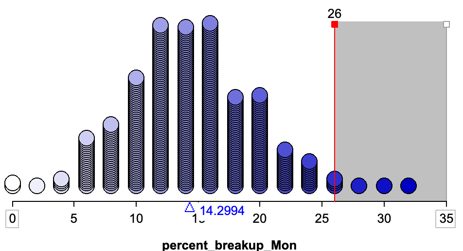
Here there are seven simulated results out of 500 that are at least as extreme as 26% (\(\geq 26%\)). The probability of obtaining a result at least as extreme as 26% if the null hypothesis were true is \(\frac{7}{500}=0.014\) (or 1.4%). We would report the \(p\)-value as \(p=0.014\).

Note, because 26% is bigger than expected if the null hypothesis were true (i.e., it is on the right-hand side of the plot), results that are more extreme than the observed result are to the right of 26%. If the observed result less than expected under the null hypothesis, more extreme results would be those smaller than the observed result.

2.12.1 Adjustment for Simulation Results

In simulation studies, we make one small adjustment to the \(p\)-value computation; we add 1 to both the numerator and denominator:

\[ p = \frac{\mathrm{number~of~results~at~least~as~extreme~as~observed~result} + 1}{\mathrm{total~number~of~simulated~results} + 1} \]

This adjustment assures that we never get a \(p\)-value of 0. Consider the \(p\)-value if our observed result would have been 32% (instead of 26%). There are 0 results that are at least as extreme as 32% (\(\geq 32%\)). Without making the simulation adjustment, we would report a \(p\)-value of 0. This implies that seeing a result at least as extreme as 32% under the null hypothesis is impossible. The problem is that we only ran 500 trials of the simulation. If we had run this simulation an infinite amount of times, we would have seen results \(\geq 32%\). So, to report a \(p\)-value of 0 is misleading. The \(p\)-value we report should be,

\[ p = \frac{0 + 1}{500 + 1} = 0.002 \]

After the adjustment, the \(p\)-value is still quite small (0.2% or 2 tenths of 1 percent), indicating that had we seen an observed result of 32%, we would say that it is not compatible with the null hypothesis.

Going back to the \(p\)-value computed from the actual observed result of 26%,

\[ p = \frac{7 + 1}{500 + 1} = 0.016 \]

We can interpret the \(p\)-value of 0.016 as indicating that the observed difference of 26% is in the outer 0.016 (1.6%) of results simulated from the hypothesized model. It is quite unlikely that we would see a result as or more extreme as 26%, if the null hypothesis were true.

2.12.2 p-Values as Evidence

Large \(p\)-values indicate that the observed data are more compatible with the results from the model, while small \(p\)-values indicate that the observed data are not very compatible with the results from the model. As researchers, our goal is often to then translate this quantitative evidence into support for the hypothesized model. For example, in the Monday breakups study, we obtained a \(p\)-value of 0.016. This means that there is a 1.6% precent chance of obtaining our observed result if the null hypothesis were true. 1.6% is a pretty low probability, whichsuggests a low degree of compatibility between the observed data (our empirical evidence) and the null hypothesis.

That said, there are no hard-and-fast rules for gauging when the evidence against a null hypothesis becomes “strong enough.” Different communities have different thresholds. And, even if there were rules about the degree of evidence needed, you would still need to evaluate other criteria such as internal and external validity evidence, and sample size. Even then, the results from a single study are not typically convincing enough for most scientists to draw definitive conclusions. It is only through consistent findings that emerge from multiple studies (which may take decades) that we may have convincing evidence about the answer to the broader scientific question.

2.12.3 Six Principles about p-Values

Because they are so ubiquitous in the research literature for any field, and because they are often misinterpreted (even by PhDs, researchers, and math teachers) it is important to be aware of what a \(p\)-value tells you, and more importantly, what it doesn’t tell you. To this end, the American Statistical Association released a statement on \(p\)-values in which it listed six principles:¹⁴

• Principle 1: \(P\)-values can indicate how incompatible the data are with a specified statistical model.
• Principle 2: \(P\)-values do not measure the probability that the studied hypothesis is true, or the probability that the data were produced by random chance alone.
• Principle 3: Scientific conclusions and business or policy decisions should not be based only on whether a \(p\)-value passes a specific threshold.
• Principle 4: Proper inference requires full reporting and transparency.
• Principle 5: A \(p\)-value does not measure the size of an effect or the importance of a result.
• Principle 6: By itself, a \(p\)-value does not provide a good measure of evidence regarding a model or hypothesis.

p-values

A \(p\)-value tells us how likely our observed result would be if the null hypothesis were true. More specifically, a \(p\)-value represents:

• The probability
• of obtaining a result at least as extreme as the observed result
• if the null hypothesis were true

To calculate a \(p\)-value from a Monte Carlo simulation, use the formula:

\[ p = \frac{\mathrm{number~of~results~at~least~as~extreme~as~observed~result} + 1}{\mathrm{total~number~of~simulated~results} + 1} \]

Resources
⏯  How to find a p-value in in TinkerPlots