# Install and load necessary packages
# install.packages(c("ggplot2", "sf", "dplyr", "rnaturalearth", "rnaturalearthdata", "ggrepel"))
library(ggplot2)
library(sf)
library(dplyr)
library(rnaturalearth)
library(rnaturalearthdata)
library(ggrepel)  # For better text placement
# Load Spain boundaries
spain <- ne_countries(scale = "medium",
                      country = "Spain",
                      returnclass = "sf")

# Load major cities
cities <- ne_download(scale = "medium",
                      type = "populated_places",
                      category = "cultural",
                      returnclass = "sf")

# Filter for cities in Spain
spain_cities <- cities %>%
  filter(ADM0NAME == "Spain") %>%
  select(NAME, LONGITUDE, LATITUDE, POP_MAX) %>%  # Keep relevant columns
  janitor::clean_names()
# Check the data
head(spain_cities)
# Plot the typography map
ggplot(data = spain) +
geom_sf(fill = "gray90", color = "white") + # Spain boundary
geom_text_repel(data = spain_cities,
aes(x = longitude, y = latitude, label = name, size = pop_max),
family = "serif", fontface = "bold", color = "darkblue", max.overlaps = 50) +
scale_size_continuous(range = c(3, 10), name = "Population") + # Scale font size by population
labs(
title = "Typography Map of Spain",
subtitle = "City names sized by population",
caption = "Source: Natural Earth | Visualization by R"
) +
coord_sf() +
theme_minimal() +
theme(
plot.title = element_text(size = 20, face = "bold", hjust = 0.5),
plot.subtitle = element_text(size = 14, hjust = 0.5),
plot.caption = element_text(size = 10, hjust = 0.5),
legend.position = "bottom"
)Save the plot as png:
ggsave("day19_typography.png",
       bg = "white",
       width = 8, height = 6, dpi = 300)
# Improved Typography Map
ggplot(data = spain) +
geom_sf(fill = "gray90", color = "white") + # Spain boundary
geom_text_repel(
data = spain_cities,
aes(x = longitude, y = latitude, label = name, size = pop_max),
family = "serif", fontface = "bold", color = "#2E86C1",
max.overlaps = 50, seed = 42
) +
scale_size_continuous(
range = c(3, 10),
breaks = c(1e6, 2e6, 3e6, 4e6, 5e6), # Add meaningful breaks
labels = scales::comma, # Human-readable labels
name = "Population (max)"
) +
labs(
title = "Typography Map of Spain",
subtitle = "City names sized by population",
caption = "Source: Natural Earth | Visualization by R"
) +
theme_minimal() +
theme(
plot.title = element_text(size = 22, face = "bold", hjust = 0.5, color = "darkblue"),
plot.subtitle = element_text(size = 16, hjust = 0.5, color = "gray40"),
plot.caption = element_text(size = 10, hjust = 0.5, color = "gray"),
legend.position = "bottom",
legend.title = element_text(size = 12, face = "bold"),
legend.text = element_text(size = 10),
panel.grid = element_blank() # Remove gridlines for a cleaner look
) +
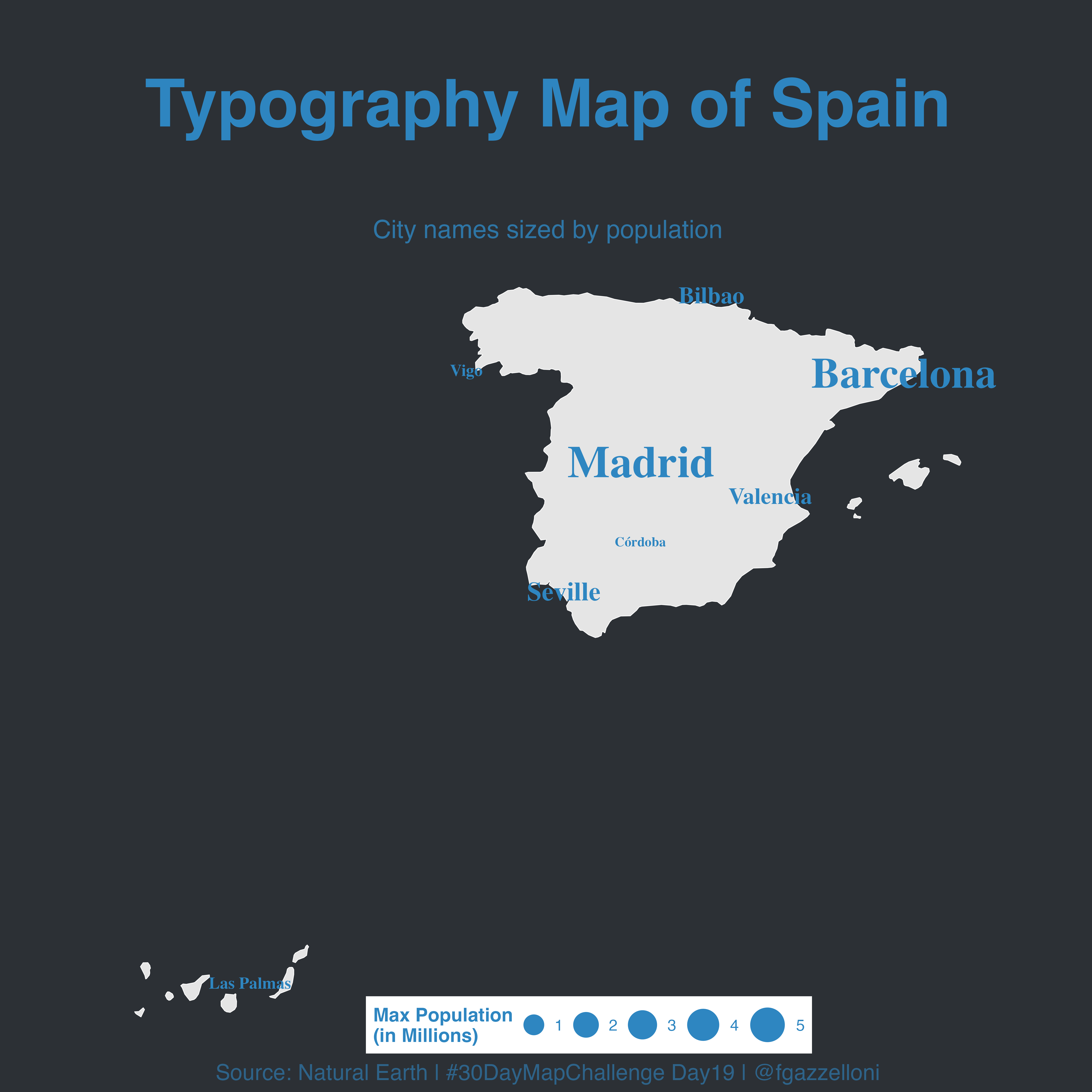
coord_sf()ggplot(data = spain) +
geom_sf(fill = "gray90",
color = "white") + # Spain boundary
geom_text_repel(data = spain_cities,
aes(x = longitude, y = latitude,
label = name,
size = pop_max),
max.overlaps = Inf,
key_glyph = "point",
family = "serif",
fontface = "bold",
color = "#2E86C1",
seed = 42) +
scale_size_continuous(range = c(3, 10),
breaks = c(1e6, 2e6, 3e6, 4e6, 5e6), # Add meaningful breaks
labels = scales::label_number(scale = 1/1e6,
suffix = ""),
name = "Max Population\n(in Millions)") +
labs(title = "\nTypography Map of Spain\n",
subtitle = "City names sized by population",
caption = "Source: Natural Earth | #30DayMapChallenge Day19 | @fgazzelloni") +
coord_sf(clip = "off") +
ggthemes::theme_map() +
theme(text = element_text(color = "#2E86C1"),
plot.title = element_text(size = 42,
face = "bold", hjust = 0.5,
color = alpha("#2E86C1", 0.99)),
plot.subtitle = element_text(size = 16, hjust = 0.5,
color = alpha("#2E86C1", 0.8)),
plot.caption = element_text(size = 14, hjust = 0.5,
color = alpha("#2E86C1", 0.6)),
legend.position = c(0.3,0),
legend.direction = "horizontal",
legend.title = element_text(size = 12, face = "bold"),
legend.text = element_text(size = 10),
panel.grid = element_blank() # Remove gridlines for a cleaner look
) Save it as png:
ggsave("day19_typography.png",
       bg = "#2c3035",scale = 1.2,
       width = 8, height = 8,
       dpi = 600)