library(tidyverse)
library(R.utils)
library(httr)
library(sf)Overview
This Ireland Map explore the population density in the area. Data is from the latest version of Kontur Population available at United Nations Humanitarian Data Exchange (HDX).
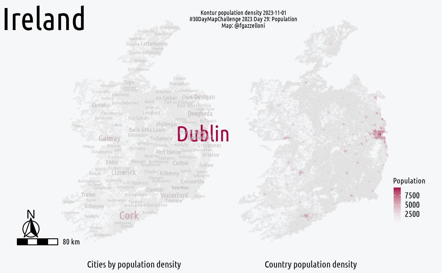
Download and unzip kontur data: 20231101
file_name <- "ireland-population.gpkg.gz"url <-"https://geodata-eu-central-1-kontur-public.s3.amazonaws.com/kontur_datasets/kontur_population_IE_20231101.gpkg.gz"
get_population_data <- function() {
res <- httr::GET(
url,
write_disk(file_name),
progress()
)
R.utils::gunzip(file_name, remove = F)
}
get_population_data()load_file_name <- gsub(".gz", "", file_name)ie_sf <- sf::st_read(load_file_name)ie_sf_lonlat <- ie_sf%>%
st_as_sf(crs = "+proj=utm +zone=29") %>%
st_transform(crs = "+proj=longlat +datum=WGS84") ie_sf_lonlat%>%
st_bbox()First raw image: Ireland population data Kontur (2023-11-01)
ggplot() +
    geom_sf(
        data = ie_sf_lonlat,
        aes(color = population),
        lwd=0.1)
ie_geo <- ie_sf_lonlat %>%
st_geometry()
hexgrid <- st_make_grid(ie_geo,
cellsize = 1e4,
what = 'polygons',
square = FALSE ## !
) %>%
st_as_sf(crs = "+proj=utm +zone=29")%>%
st_transform(crs = "+proj=longlat +datum=WGS84")
hexgrid2 <- hexgrid[c(unlist(st_contains(ie_geo, hexgrid)),
unlist(st_overlaps(ie_geo, hexgrid))) ,] List of Cities, boroughs and towns up to 2014:
ireland_cities_tb <- read.csv("data/ie.csv")
ireland_cities_tb%>%head
ie_cities_sf <- ireland_cities_tb%>%
st_as_sf(coords=c("lng","lat"),crs="+proj=longlat +datum=WGS84")ie_cities_sf%>%summary()
ie_cities_sf<-ie_cities_sf%>%
filter(!is.na(population))Fonts
library(sysfonts)
library(showtext)
sysfonts::font_add_google("Ubuntu Condensed","Ubuntu Condensed")
text<-"Ubuntu Condensed"
showtext::showtext_auto()
showtext::showtext_opts(dpi=320)
library(ggspatial)set.seed(20231129)
p <- ggplot() +
geom_sf(data = ie_sf_lonlat,
mapping=aes(color = population),
lwd=0.1)+
scale_color_gradient(low = alpha("#cdbdcc",0.01),
high = "#a60845",
guide = "none")+
ggnewscale::new_scale_color()+
geom_sf_text(data=ie_cities_sf,
mapping=aes(label=city,
color=population,
size=population),
show.legend = F,
family=text,
check_overlap = T)+
scale_color_gradient(low = alpha("#c2bfbf",0.9),high = "#a60845",)+
coord_sf(clip="off")+
ggthemes::theme_map()+
theme(text=element_text(family=text),
plot.caption = element_text(hjust = 0.5),
legend.background = element_blank(),
legend.position = "none",
legend.key.size = unit(7,units = "pt"),
legend.text = element_text(size=7))+
ggspatial::annotation_north_arrow(location = "bl",
which_north = "true",
pad_x = unit(-0.9, "cm"),
pad_y = unit(0.4, "cm"),
height = unit(0.8, "cm"),
width = unit(0.8, "cm"),
style = north_arrow_fancy_orienteering)+
ggspatial::annotation_scale(pad_x = unit(-0.9, "cm"),
height = unit(0.18, "cm"),
text_family=text,
text_cex = 0.5)+
labs(caption="Cities by population density")
pp1<- ggplot() +
geom_sf(data = ie_sf_lonlat,
mapping=aes(color = population),
lwd=0.5)+
scale_color_gradient(low = alpha("#cdbdcc",0.01),high = "#a60845",guide=guide_colorbar(title = "Population"))+
labs(caption="Country population density")+
ggthemes::theme_map()+
theme(text=element_text(family=text),
plot.caption = element_text(hjust = 0.5),
legend.background = element_blank(),
legend.position = c(0.95,0.1),
legend.key.size = unit(6,units = "pt"),
legend.title = element_text(size=6.1),
legend.text = element_text(size=7))
p1library(cowplot)
ggdraw()+
draw_plot(p,x=-0.2,y=0)+
draw_plot(p1,x=0.2,y=0)+
draw_label(label="Ireland",
x=0.1,y=0.93,
size=25,
fontfamily=text,
fontface = "bold")+
draw_label(label="Kontur population density 2023-11-01\n#30DayMapChallenge 2023 Day 29: Population\nMap: @fgazzelloni",
x=0.55,y=0.93,
size=5,
fontfamily=text,
fontface = "bold")
ggsave("day29_population.png",bg="#f6f7f9")