Chapter 3 Agent-based modeling

R can be used in order to simulate agents’ behaviors in virtual environments. In the following I will introduce you to what this can look like. In the end, there are further resources where you can find more ABM examples in R and also some theoretical background.

3.1 Building an ABM: Schelling model

When designing an ABM from scratch, we need to take a bunch of things into account. A structural way to think about this is in terms of a flow chart.

In the first part, we need to create the agents and their world. We need to think about parameters that need to be specified and how they can be implemented in their code. Thereafter, the actual agent (inter)actions take place. In the end, we can evaluate the (macro) outcomes and check for robustness etc. In this part of the script, it’s going to be about the former two steps.

When writing an ABM in R, I would advise you to write functions for each step in the flow chart and run the entire thing in a for loop or while loop.

3.1.1 Recap: functions, if…else, loops, and matrices

Building blocks for ABMs in R are custom functions (since you want your agents to do things…), flow control (…under certain conditions…), and loops (…several times in a row). Matrices are handy to implement a cellular automaton.

3.1.1.1 Functions

When you define functions in R, you need to follow a certain structure:

function_name <- function(argument_1, argument_2, argument_n) {
  function body
}

The function_name is the thing you will call (e.g., mean()). In general, it should be a verb, it should be concise, and it should be in_snakecase.
The arguments are what you need to provide the function with (e.g., mean(1:10)).
The function body contains the operations which are performed to the arguments. It can contain other functions as well – which need to be defined beforehand (e.g., sum(1:10) / length(1:10))). It is advisable to split up the function body into as little pieces as you can.

3.1.1.2 Loops

With ABMs you often want to loop until a certain condition is met. This is where while loops come in handy.

The basic structure of while loops is as follows:

while (condition) {
  code
}

Alternatively, you can also do a for loop with a pre-defined set of runs and a break() condition:

for (i in seq_along(seq(number_of_iterations))) {
  do_something_i_times
  
  if break_condition_is_met break
}

Note in both cases that you need to pre-allocate space for your loop to run smoothly for instance by pre-defining a list with vector(mode = "list", length = number_of_iterations)

3.1.1.3 Flow control

Sometimes you want your code to only run in specific cases. A generalized solution for conditionally running code in R are if statements. They look as follows:

if (conditional_statement evaluates to TRUE) {
  do_something
}

They also have an extension – if…else:

if (conditional_statement evaluates to TRUE) {
  do_something
} else {
  do_something_else
}

3.1.1.4 Matrix

A matrix is a multidimensional vector. We need it for building a cellular automaton like the one used by Schelling (1971). It is created using `matrix(values, nrow = number_of_rows, ncol = number_of_columns). Thereafter, the

matrix(1:10, nrow = 2) # by default, it's filled by columns

##      [,1] [,2] [,3] [,4] [,5]
## [1,]    1    3    5    7    9
## [2,]    2    4    6    8   10

matrix(1:10, nrow = 2, byrow = TRUE) # can be also filled by rows

##      [,1] [,2] [,3] [,4] [,5]
## [1,]    1    2    3    4    5
## [2,]    6    7    8    9   10

example <- matrix(sample(0:2, 10*10, replace = TRUE, prob = c(0.4, 0.3, 0.3)), ncol = 10) # probably more useful for a cellular automaton

A matrix can be visualized by transforming it to an image.

image(example, col = c("black","red","green"), axes = FALSE)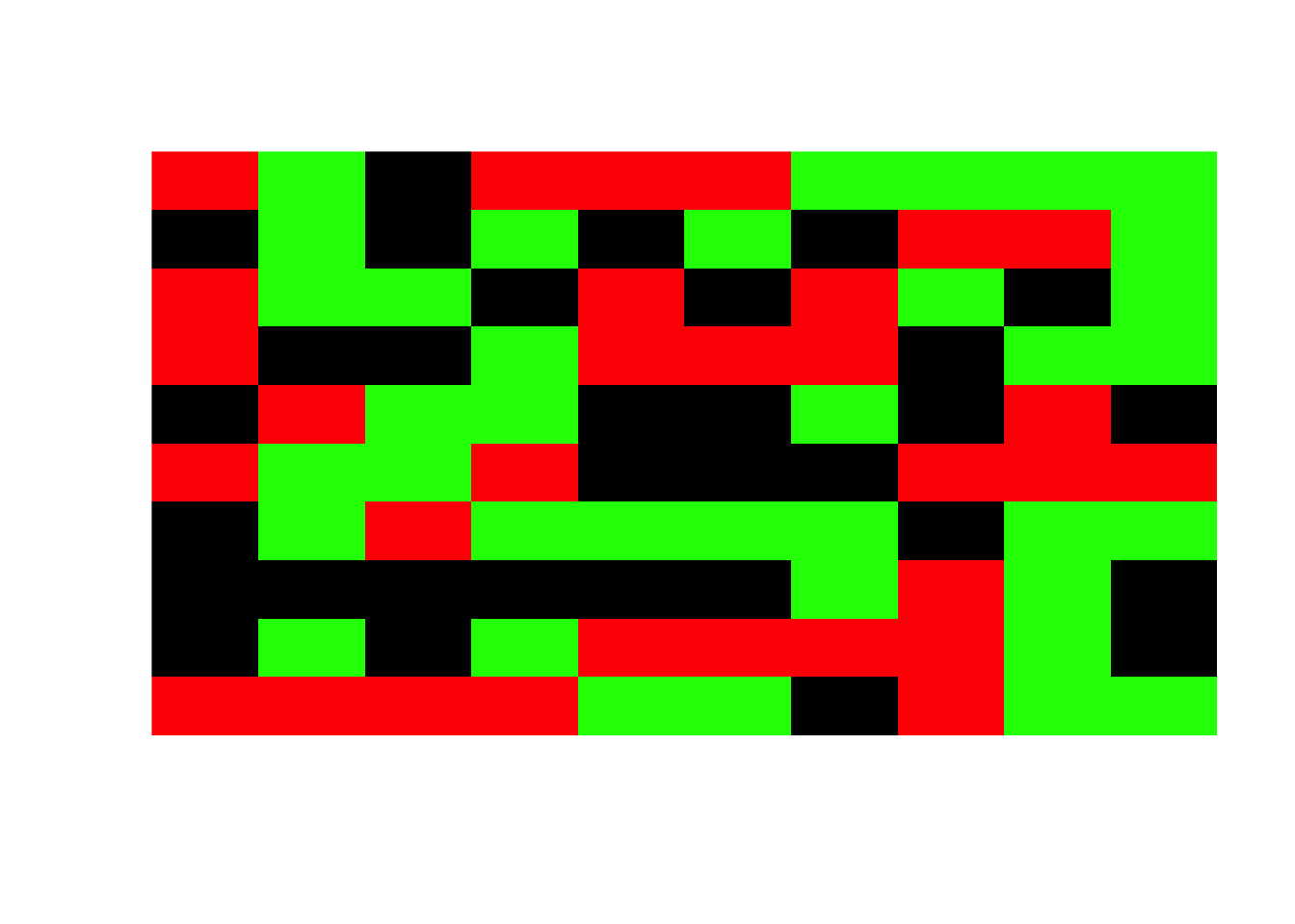

Note that you can index a matrix using [row, column].

3.1.2 Schelling model

Let’s build a Schelling model together. The inspiration for parts of the code come from this blog post – I tried to write the code in a cleaner fashion though.

The steps we will program today are the follwoing:

Initialization:
- Create field with n x n dimensions
- Create agents with certain attributes and put them on the field
- Determine happiness criterion
Simulation
- Determine each agent’s happiness level
- Move unhappy agents to empty field
- Repeat until time is up or all agents are happy

3.1.2.1 Initialization

Build a 25x25 matrix. It should contain 0s (for unoccupied field), 1s (color 1), and 2s (color 2). Make sure to wrap it in a function with different parameters for the share of different colors. Let R print an image() of it.

build_world <- function(dimensions, share_free, share_col_1, share_col_2) {
  if (share_free + share_col_1 + share_col_2 != 1) stop("shares need to add up to 1.")
  
  matrix(sample(0:2, dimensions^2, replace = TRUE, prob = c(share_free, share_col_1, share_col_2)), 
         ncol = dimensions)
}
image(build_world(dimensions = 25, share_free = 0.5, share_col_1 = 0.25, share_col_2 = 0.25), axes = FALSE)

Determine the initial happiness criterion as 0.4 – you will need to feed it to the executing functions later. The happiness criterion is the least share of neighbors surrounding an individual that is of the same color as the agent itself.

happiness_criterion <- 0.4

3.1.2.2 Action

Build a function that determines each agent’s happiness (hint: you can use a nested for loop for looping through the matrix).
1. write a function to determine one agent’s neighbors (as determined through their coordinates [row, col] – Moore neighborhood, i.e., all 8 neighbors)
2. determine whether the agent is happy (is the share of same-value neighbors above the threshold? – hint: exclude the empty fields first and stop the function if a person does not have neighbors – then the person is automatically happy). Moreover, determine the share of same-value agents in each agent’s environment.
3. loop over all coordinates to check whether the agents are happy; store the results in a tibble with the following cells: row, column, happiness (NA if free spot, 0 if unhappy, 1 if happy)
4. write a function to determine the share of happy agents.

build_world(dimensions = 25, share_free = 0.5, share_col_1 = 0.25, share_col_2 = 0.25)
coordinates <- c(2,1)
dimensions <- 25
#a
get_neighbors <- function(coordinates, dimensions) {
  if (coordinates[1] > dimensions) stop("invalid value for coordinates[1]")
  if (coordinates[2] > dimensions) stop("invalid value for coordinates[2]")
  
  expand_grid(dim_1 = (coordinates[1] - 1):(coordinates[1] + 1),
              dim_2 = (coordinates[2] - 1):(coordinates[2] + 1)) %>% 
    filter(dim_1 > 0,
           dim_2 > 0,
           dim_1 <= dimensions,
           dim_2 <= dimensions,
           !(dim_1 == coordinates[1] & dim_2 == coordinates[2]))
}

#b
determine_same_share <- function(coordinates, field_matrix) {
  own_value <- field_matrix[coordinates[1], coordinates[2]]
  
  if (own_value == 0) return(NA_real_)
  
  neighbors <- get_neighbors(coordinates, dimensions = nrow(field_matrix))
  map2(neighbors[[1]], neighbors[[2]], ~field_matrix[.x, .y]) %>% 
    reduce(c) %>% 
    enframe(name = NULL, value = "neighbor") %>% 
    mutate(own_value = own_value) %>% 
    filter(neighbor != 0) %>% 
    mutate(same_type = case_when(own_value == neighbor ~ TRUE,
                                 TRUE ~ FALSE)) %>% 
    pull(same_type) %>% 
    mean()
}
# c
coordinate_tbl <- expand_grid(dim_1 = 1:25, dim_2 = 1:25) %>% 
  mutate(same_share = NA_real_,
         happiness_ind = NA_real_)

for (i in seq_along(coordinate_tbl$same_share)) {
  
  coordinate_tbl$same_share[i] <- determine_same_share(coordinates = c(coordinate_tbl$dim_1[i],
                                                                       coordinate_tbl$dim_2[i]),
                                                       field_matrix = field_matrix)
  if (is.nan(coordinate_tbl$same_share[i]) == TRUE) coordinate_tbl$happiness_ind[i] <- 1
  if (is.nan(coordinate_tbl$same_share[i]) == TRUE) next
  if (is.na(coordinate_tbl$same_share[i]) == TRUE) next
  
  if (coordinate_tbl$same_share[i] >= happiness_criterion) {
    coordinate_tbl$happiness_ind[i] <- 1
  }else{
    coordinate_tbl$happiness_ind[i] <- 0
  }
}

# d
determine_happy_share <- function(coordinate_tbl) {
  mean(coordinate_tbl[["happiness_ind"]], na.rm = TRUE)
  }

Make the unhappy cells “move” to a free spot. Make sure that the agents will be randomized before so that there is no spatial bias (hint: pingers::shuffle()).

unhappy_ones <- coordinate_tbl %>% 
  filter(happiness_ind == 0) %>% 
  pingers::shuffle()
free_spots <- coordinate_tbl %>% 
  filter(is.na(happiness_ind)) %>% 
  pingers::shuffle()

move_agents <- function(unhappy_ones, free_spots, field_matrix) {
  i <- 1
  while (i <= nrow(unhappy_ones)) {
    field_matrix[free_spots$dim_1[i], free_spots$dim_2[i]] <- field_matrix[unhappy_ones$dim_1[i], unhappy_ones$dim_2[i]]
    field_matrix[unhappy_ones$dim_1[i], unhappy_ones$dim_2[i]] <- 0
    if(i == nrow(free_spots)) {
      unhappy_ones %<>% slice(., (i + 1):nrow(.))
      free_spots <- which(field_matrix == 0, arr.ind = TRUE) %>% 
        as_tibble() %>% 
        select(dim_1 = row,
                 dim_2 = col) %>% 
        pingers::shuffle()
      i <- 1
      }
    i <- i + 1
  }
  field_matrix
}

Put the functions in a while loop that runs as long as you want or until all agents are satisfied.

get_own_value <- function(coordinate_a, coordinate_b, matrix_name) matrix_name[coordinate_a, coordinate_b]

run_schelling <- function(max_steps = 500, 
                          dimensions = 25,
                          share_free = 0.2, 
                          share_col_1 = 0.4, 
                          share_col_2 = 0.4,
                          happiness_criterion = 0.4) {
  current_step <- 1
  share_unhappy <- 1
  field_matrix <- build_world(dimensions, share_free, share_col_1, share_col_2)
  report_tbl <- tibble(
    step = 1:max_steps,
    unhappy_ones = NA_integer_
  )
  #image_list <- vector(mode = "list", length = max_steps/3 + 1)
  agent_list <- vector(mode = "list", length = max_steps)
  coordinate_tbl <- expand_grid(dim_1 = 1:dimensions, dim_2 = 1:dimensions) %>% 
    mutate(happiness_ind = NA_real_,
           same_share = NA_real_)
  
  while (current_step <= max_steps & share_unhappy > 0) {
    
    for (i in seq_along(coordinate_tbl$happiness_ind)) {
        coordinate_tbl$same_share[i] <- determine_same_share(coordinates = c(coordinate_tbl$dim_1[i],
                                                                         coordinate_tbl$dim_2[i]),
                                                             field_matrix = field_matrix)
      
      if (is.nan(coordinate_tbl$same_share[i]) == TRUE) coordinate_tbl$happiness_ind[i] <- 1
      if (is.nan(coordinate_tbl$same_share[i]) == TRUE) next
      if (is.na(coordinate_tbl$same_share[i]) == TRUE) next
    
      if (coordinate_tbl$same_share[i] >= happiness_criterion) {
        coordinate_tbl$happiness_ind[i] <- 1
      }else{
        coordinate_tbl$happiness_ind[i] <- 0
      }
    }
    
    agent_list[[current_step]] <- coordinate_tbl %>% 
      mutate(own_value = map2_dbl(dim_1, dim_2, get_own_value, field_matrix))
    
    share_unhappy <- 1 - mean(coordinate_tbl %>% filter(!is.na(same_share)) %>% pull(happiness_ind), na.rm = TRUE)
    
    unhappy_ones <- coordinate_tbl %>% 
      filter(happiness_ind == 0) %>% 
      pingers::shuffle()
    
    free_spots <- coordinate_tbl %>% 
      mutate(own_value = map2_dbl(dim_1, dim_2, get_own_value, field_matrix)) %>% 
      filter(own_value == 0) %>% 
      pingers::shuffle() %>% 
      select(1:2)
  
    field_matrix <- move_agents(unhappy_ones, free_spots, field_matrix)
    
    report_tbl$unhappy_ones[current_step] <- round(share_unhappy, 3)
    #print(str_c("step: ", current_step, "; share of unhappy agents: ", round(share_unhappy, 3)))
    
    #if (current_step == 1 | current_step %% 3 == 0) image_list[[current_step]] <- image(field_matrix, axes = FALSE)
    
    current_step <- current_step + 1
  }
  list(report_tbl %>% drop_na(), agent_list %>% compact())
}

test <- run_schelling(max_steps = 5)

And voilà, your first ABM.

3.1.3 Results

Let’s make some checks for how our input variables affect our output. In order to do so, we need to run the simulations often with all different kinds of parameters. For a first check, I will do so just using a grid of input variables. As the simulations can run independently from each other, I can use the furrr package. This allows you to run purrr functions in parallel.¹

library(tidyverse)
#library(furrr)
input_table <- expand_grid(
  max_steps = 50,
  dimensions = c(25, 50),
  share_col_1 = seq(0.2, 0.4, by = 0.1),
  happiness_criterion = seq(0.2, 0.8, by = 0.2)
) %>% 
  mutate(share_col_2 = share_col_1,
         share_free = 1 - (share_col_1 + share_col_2)) %>% 
  filter(share_free > 0.1)

#plan(multisession, workers = 8)

#results <- future_pmap(input_table,
#                       run_schelling, 
#                       .options = furr_options(seed = 123))

I have run the simulations on a server, so let’s look at the results. The list contains one tibble which contains the share of unhappy agents at each step. Moreover, it contains another list with tibbles that consist of all agents and their happiness-score as well as their color.

results <- read_rds("data/results_schelling.rds")
#glimpse(results[[1]][[1]])

Let’s look at the results in a structured manner. For this, we create new columns in the initial parameter table which we can then use for both regression analysis and visual inspection. Our dependent variables are overall segregation and the share of happy agents. The former can be measured by the final average share of same-type agents.

Does the dimensionality make any tangible difference with regard to how fast all agents become happy? Look at different dimension-groups using facets, differentiate between happiness criteria.

input_table_agent <- input_table %>% 
  rowid_to_column("run") %>% 
  left_join(results %>% map(pluck, 1) %>% bind_rows(.id = "run") %>% mutate(run = run %>% as.integer())) %>% 
  mutate(avg_happiness = 1-unhappy_ones) %>% 
  group_by(happiness_criterion, step, dimensions) %>% 
  summarize(happy_avg = mean(avg_happiness, na.rm = TRUE)) %>% 
  ungroup() %>% 
  mutate(step = as.double(step))

## Joining, by = "run"

## `summarise()` has grouped output by 'happiness_criterion', 'step'. You can override using the `.groups` argument.

ggplot(input_table_agent) +
  geom_line(aes(x = step, y = happy_avg, color = as_factor(happiness_criterion))) +
  facet_grid(. ~ dimensions) +
  labs(color = "happiness")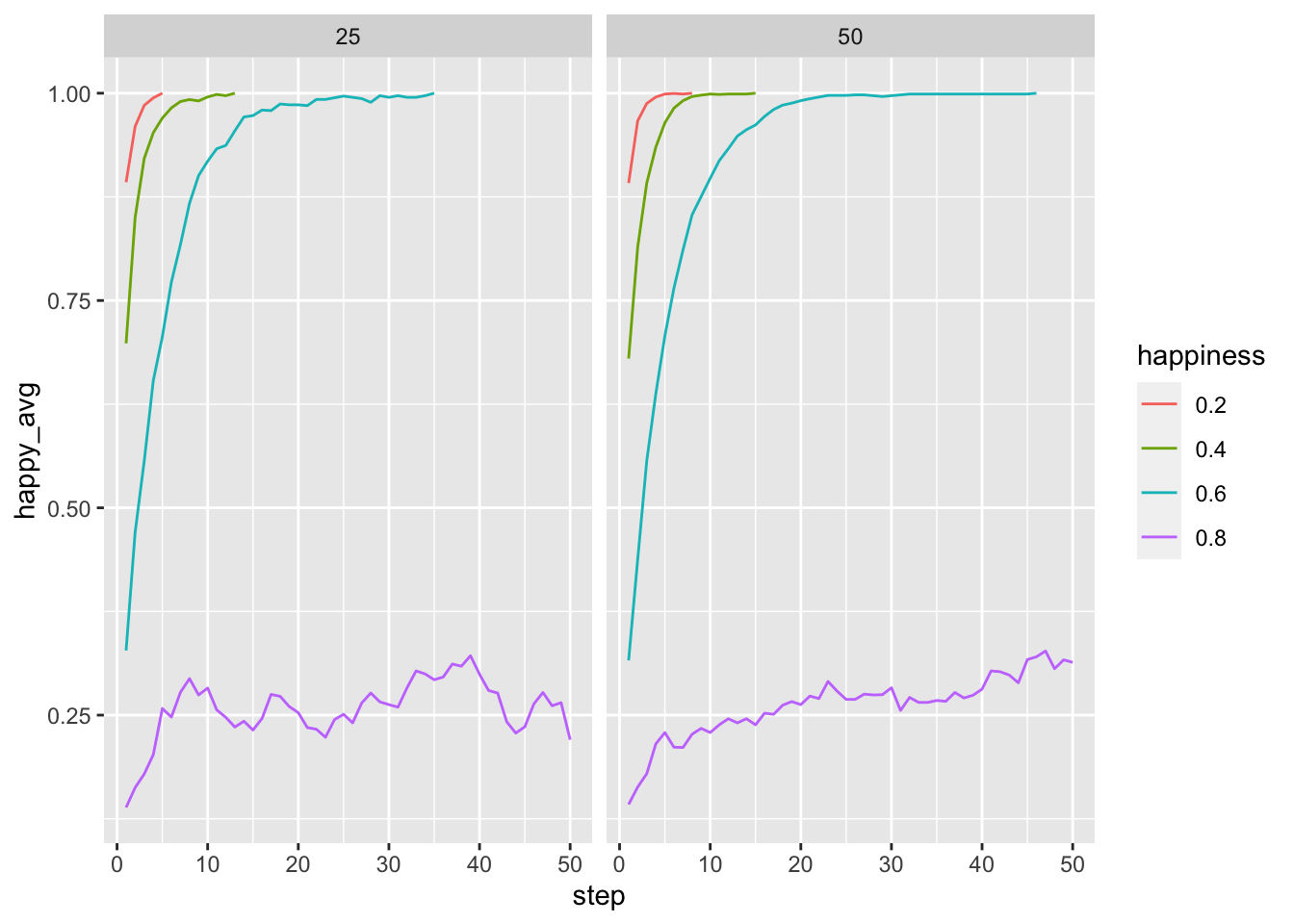

How do the different shares affect final segregation?

input_table_w_result <- input_table %>% 
  mutate(happiness_ind = map_dbl(results, ~.x[[2]][length(.x[[2]])] %>% 
                                    pluck(1) %>% 
                                    pull(happiness_ind) %>% 
                                    mean(na.rm = TRUE)),
         same_share = map_dbl(results, ~.x[[2]][length(.x[[2]])] %>% 
                               pluck(1) %>% 
                               pull(same_share) %>% 
                               mean(na.rm = TRUE)))

ggplot(input_table_w_result) +
  geom_point(aes(x = share_col_1, y = same_share))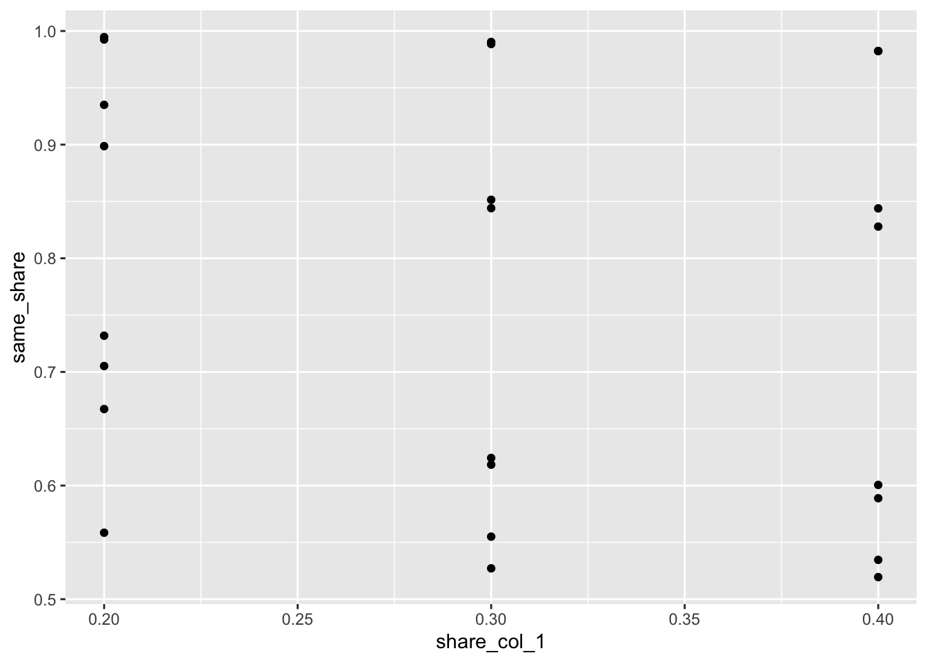

Let’s disentangle the influence the different parameters have on the outcome.

Build a regression model that has final segregation as dependent variable and all the parameters as input variables. Note: do only include one share_* variable due to multicollinearity.

model_1 <- lm(same_share ~ dimensions + share_col_1 + happiness_criterion, data = input_table_w_result) %>% 
  summary()

Well, in the former model, we still had the runs with the happiness-criterion of 0.8. Those destroy our results.

model_1_1 <- lm(same_share ~ dimensions + share_col_1 + happiness_criterion, data = input_table_w_result %>% filter(happiness_criterion < 0.8)) %>% 
  summary()

Build a regression model that has the eventual number of steps as dependent variable and all the parameters as input variables. Note: only include one share_* variable due to multicollinearity.

model_2 <- input_table %>% 
  rowid_to_column("run") %>% 
  left_join(results %>% map(pluck, 1) %>% bind_rows(.id = "run") %>% mutate(run = run %>% as.integer())) %>% 
  add_count(run, name ="n_steps") %>% 
  lm(n_steps ~ dimensions + happiness_criterion + share_col_1, data = .) %>% 
  summary()

## Joining, by = "run"

3.2 How to report ABMs – the ODD protocol

The most common way to report an ABM is the so called ODD protocol. ODD stands for “Overview, Design concepts, Details.” It was introduced by Grimm et al. (2006) and recently updated (Grimm et al. 2020). A comprehensive overview of the ODD protocol can be found on the web site of the Network for Computational Modeling in Social and Ecological Sciences (CoMSES).

The overarching goals of the ODD protocol are to make scientists’ lives easier. It strives to facilitate the conceptualization of the model for the user (“what decisions do I have to make?”) as well as the reproduction of models for future validation. Standardized descriptions help readers to comprehend the different components.

The components are the following:

Purpose and patterns
Entities, state variables, and scales
Process overview and scheduling
Design concepts
Initialization
Input data
Submodels

3.2.1 Baldassarri and Bearman (2007) ODD’ed

In the following, I will go through the components with examples from the ABM in Baldassarri and Bearman (2007). Thereby, I will also showcase the code that corresponds to the respective components. This highlights how the protocol serves the researcher as a tool to conceptualize and develop an ABM from scratch.

3.2.1.1 Purpose and patterns

In the first step, researchers need to justify the purpose the model. This encompasses not only stating the research question, but also what general purpose the model is supposed to serve for. Those high-level purposes are not necessarily perfectly distinct and a model might serve for more than one. However, when you construct a model, you should clearly think of one purpose and garner it towards this purpose.

Some of the most important high-level purposes of ABMs are prediction (of an outcome), explanation (of phenomena through tangible causal chains consisting of mechanisms), description (of the components that matter in a particular case), theoretical exposition (hypothesis testing), illustration (of an idea or theory), analogy (to illustrate a way you could think about a phenomenon – such as opinion spreading through models from epidemiology), and social learning (modeling the evolution of people’s (shared) understandings) (illustrations and more can be found in Edmonds et al. 2019).

The “patterns” part of the first component refers to the (real-world) phenomenon you strive to explain. It can be seen as a set of criteria that help you in assessing whether the model is realistic enough. The patterns can be derived from observations on either the micro- or macro level in the real world or inductively from the literature. For instance, the pattern we wanted to observe in the diffusion model was the S-shaped curve we know from real-world diffusion processes, or in the Schelling model clearly segregated neighborhoods.

A clearly formulated purpose and pattern part helps the reader with deciding independently whether they deem the model a success or not. Moreover, it helps the researcher to decide what is relevant for their model and what not – and, hence, what they need to include. It is advisable to clearly link the model’s outcomes/results to the question. This will also inform your decision on what to report and how. Relevant terms need to be sufficiently specified. Alternative use-cases of the model need to be included (e.g., diffusion models can be useful for modeling epidemics as well as rumors or trends). Do not get into the specifics of your model already, this will come in the later parts of the ODD protocol. And, finally, formulate patterns in such a way that they are testable: how can you reliably (statistically) determine whether they are present or not? Also, it needs to be motivated why you assume them to be of relevance for your model. This usually stems from empirical observation.

Purpose and pattern of Baldassarri and Bearman (2007):

They set out to determine the mechanisms behind two empirical paradoxes:

“The first is the simultaneous presence and absence of political polarization—the fact that attitudes rarely polarize, even though people believe polarization to be common. The second is the simultaneous presence and absence of social polarization—the fact that while individuals experience attitude homogeneity in their interpersonal networks, these networks retain attitude heterogeneity overall.” (p. 784)

Therefore, the patterns they are searching for are homogeneous individual discussion networks, whereas the social structures themselves remain heterogeneous. Moreover, they claim that there are topics (so-called “takeoff issues”) that garner the lion share of attention, leading to no polarization with regard to other topics.

3.2.1.2 Entities, state variables, and scales

The entities of the model are the objects that in their entirety comprise the model. Objects are usually of different kinds and multitude. Typically there are the following kinds of entities in there: spatial units such as grid cells or, more abstractly speaking, actors’ position in a network; the actors (agents) themselves; agent collectives/groups; the environment, such as time trackers, observers (of the distribution of agents). The inclusion of entities should be theoretically motivated and needs to be justified.

State variables are the attributes of the different entities. Those can be used to distinguish entities of the same kind (e.g., color in the Schelling model) or track changes over time (e.g., position of the agent in the Schelling model). When including state variables, one also has to descriebe them in further detail: what are they representing; are they dynamic; what’s the values they can take on and what type are they of. It usually makes sense to perform those descriptions in a table. Note the difference between state variables and parameters: state variables capture the entity’s state over time or are used to distinguish entities. Therefore, agents’ gender is a state variable, the happiness threshold in the Schelling model is a parameter. If a value is drawn from, say, a normal distribution as the opinion value in Baldassarri and Bearman (2007), the agent’s value is captured as a state variable. In this case, the parameters would be the characteristics of the normal distribution (mean and standard deviation). State variables should be as “low-level” as possible. If a value is derived from other state variables, it is no state variable in itself. Also, do not mention why those variables might change.

When thinking about which state variables to include, ask yourself: “if you want (as modelers often do) to stop the model and save it in its current state, so it can be re-started in exactly the same state, what is the minimum information you must save? Those essential characteristics of each kind of entity are its state variables.” (Grimm et al. 2020, S1: 9)

Scales are referring to the extent of the model: its spatial and temporal scale. What does one time step mean? What does one square grid cell refer to? Also, justify your decision for a certain decision. This must only be included if it applies. However, you should give an abstract discussion (e.g., in the Schelling model cells represent households and one step is one move, so roughly a couple of months). This makes the model more tangible.

Note that in this part you should not discuss the model processes and behaviors. Stick to the entities, state variables, and scales.

Entities, state variables, and scales in Baldassarri and Bearman (2007):

The entities are the 100 individual actors. Their state variables are issue interest/opinion towards issues and the (perceived) distance to other actors $\lambda$ . Scale-wise, the simulations will run for 500 steps and actors can communicate to a certain number of actors (up to ~12) during each time step.

library(tidyverse)
actor_list <- vector(mode = "list", length = 100L)
for (i in seq_along(actor_list)){
  temp <- rnorm(n = 4, mean = 0, sd = 33.3)
  temp[temp > 100] <- 100
  actor_list[[i]] <- temp
}

euclidean <- function(a, b) sqrt(sum((a - b)^2)) %>% as.double()

a <- 1:3
b <- 1:6

distance_df <- expand_grid(a = 1:100, b = 1:100) %>% 
  filter(a != b) %>% 
  mutate(euclidean_vec = NA_real_)

for (i in seq_along(distance_df$a)) {
  distance_df$euclidean_vec[[i]] <- euclidean(actor_list[[distance_df$a[[i]]]], actor_list[[distance_df$b[[i]]]])
}

3.2.1.3 Process overview and scheduling

Describe the processes (actions) within the model and the order in which they are performed. This can happen in fairly coarse terms. Also specify the schedule (in which order the processes are performed). When you code your model, you can easily interpret and implement the singular steps as functions. This will make your code very readable and comprehensive.

An action is described in terms of an entity that executes a process or behavior that changes certain state variables. Those processes within the action are performed in a certain order. Those actions are listed in submodels, which are to be described in further detail in a later part.

You need to include everything that is completed at each time step, and describe all variables that might be affected by that. Moreover, if an action is performed by more than one entity, you need to specify the order. The schedule summary has to be clear about when the variables are updated (it helps to look at the former section where you specified all the state variables).

Furthermore, you should explain why you included those processes and scheduled them in the manner you did. Feel free to provide a flow chart or pseudo code to illustrate the schedule.

Your model might contain discrete events, an intervention or so. Make sure to include how those are scheduled.

Process overview and scheduling in Baldassarri and Bearman (2007):

Each round a random sample of potential interlocutors is drawn for each actor. The size of the sample is proportional to the actor’s overall level of interest. This follows from the assumption that “the more one is committed to a cause, the more likely one is to start a conversation.” (p. 790) People have a tendency for homophily with regard to their social contacts. Hence, actors choose the ones they want to deliberate with based on their overall ideological proximity. However, they do not exclusively communicate with the ones they are similar to, there is still some room for communication with ideologically dissimilar ones – those interactions happen less often though. In the beginning, actors do not know about others’ ideological stance. They learn it through interaction.

The process of interpersonal influence looks as follows: first, the issue for discussion is chosen based on the cumulative interest of both actors. Second, the new opinions of both actors towards the chosen issue are computed and modified. Those can either be reinforced or become more neutral. Individuals which share the same position on the issue reinforce each others’ opinions, whereas people with diverging views may either find a compromise (if they are similar on other dimensions), leading to opinions closer on the ideology scale, or indulge in further conflict, where their opinions grow further apart from each other. This affects the new overall level of interest of both users as well as their ideological distance between them.

3.2.1.4 Design concepts

Here, you need to relate your model to 11 common concepts in ABM. This is useful to place it within the ABM literature. A more conclusive description can be found in the supplemental material to Grimm et al. (2020).

basic principles: how does the model relate to existing approaches, how are they implemented or taken into account? Is there new literature included that has not been implemented yet?
emergence: which model results stem from which mechanisms, which are imposed by rules, why are some results more or less emergent?
adaptation: what decisions are agents making in response to what stimuli; which alternatives can they choose from, the variables that affect the decision, how do they make the decision – direct or indirect objective seeking
learning: if agents change their decision-making based on prior “experience”
prediction: do agents try to foresee future outcomes and adapt their decisions to this
sensing: does an agent get to know other entities state variables; usually it’s assumed that they have full information, but the sensing process might give them not perfect information
interactions: are agents interacting and how (direct or mediated)?
stochasticity: if you draw numbers at any place from some sort of stochastic distribution – why and how?
collectives: groups of agents – either through (implicit) emergence or through determination (e.g., political parties); are they included, how, and what are the consequences?
observation: how is information collected and summarized/analyzed?

Design concepts of Baldassarri and Bearman (2007):

basic principles: “Models that involve dynamics of interpersonal influence differ broadly in their scope, ranging from the study of dynamics of ideological polarization (Hegselmann and Krause 2002; Macy et al. 2003; Nowak et al. 1990), collective action (Kim and Bearman 1997), and collective decision-making (Marsden 1981) to the persistence of cultural differences (Axelrod 1997) and political disagreement (Huckfeldt, Johnson, and Sprague 2004). Our goal has been to deploy a model of interpersonal influence sensitive to dynamics of political discussion, where actors hold multiple opinions on diverse issues, interact with others relative to the intensity and orientation of their political preferences, and through evolving discussion networks shape their own and others’ political contexts. In the model, opinion change depends on two factors: the selection of interaction partners, which determines the aggregate structure of the discussion network, and the process of interpersonal influence, which determines the dynamics of opinion change.” (p. 788)
emergence: through agents’ interactions and the opinion changes those might encompass
adaptation: agents have an engrained tendency to prefer similar others and avoid conflict
learning: agents learn about their peers’ opinions which subsequently alters the probibility of contact
prediction: not applicable
interactions: agents communicate bidirectional – discourse leads to opinion changes in both agents
sensing: agents have full information on other agents’ ideology
stochasticity: agents’ interlocutors are chosen at random, the number of potential interlocutors is based on political interest though; a Bernoulli process determines, whether they actually talk to each other, depending on their ideological similarity; the initial distribution of opinions is determined through a normal distribution
collectives: not applicable
observation: state variables are updated after every interaction; eventually, takeoff cases are identified through the Herfindahl-Hirschman index; networks are qualitatively interpreted with regard to the dominating topics; an index of polarization is computed based on the dispersion and bimodality of the distribution of opinions to uncover relative levels of polarization; modularity is used to assess how polarized the network is (i.e., how well partitioning the network into two clusters works); finally, it is determined how homogeneous the networks for each individual appear and whether this differs for takeoff and non-takeoff cases.

3.2.1.5 Initialization

In the final three parts of the ODD protocol, you really need to go into detail with the model. In the first part, you describe the initialization: what are the entities that are created, how many of them – and why this number, and what values are given to state values. Perhaps, are there locations/collectives set; is there specific data used to create the agents, the space, or the parameters beforehand, where do they come from and are there potential pitfalls/biases? Are there different initialization scenarios – if so, why?

In here, the most important thing is the why: what drives your decisions here. Include relevant references and justify your decisions.

Initialization in Baldassarri and Bearman (2007):

the model consists of 100 actors. Those hold opinions on 4 issues. The authors do not provide justifications for why they chose exactly 100 actors and 4 issues. Those opinions are not only opinions but also serve as indicators of the actor’s interest towards the particular topic. They argue that this is a reasonable assumption since prior research has consistently shown that people with stronger interest in a topic also usually have stronger opinions. Opinions on each topic are independent from each other and drawn from a normal distribution with mean 0 and standard deviation 33.3. Moreover, each agent gets an initial value for the perceived distance to their peers. It’s the demeaned euclidean distance (normalized by division by max(euclidean_distance)) between all actors.

There are no different initialization scenarios.

library(tidyverse)
library(magrittr)
actor_list <- vector(mode = "list", length = 100L)
for (i in seq_along(actor_list)){
  temp <- rnorm(n = 4, mean = 0, sd = 33.3)
  temp[temp > 100] <- 100
  actor_list[[i]] <- temp
}

euclidean <- function(a, b) sqrt(sum((a - b)^2)) %>% as.double()

a <- 1:3
b <- 1:6

distance_df <- expand_grid(a = 1:100, b = 1:100) %>% 
  filter(a != b) %>% 
  mutate(euclidean_vec = NA_real_)

for (i in seq_along(distance_df$a)) {
  distance_df$euclidean_vec[[i]] <- euclidean(actor_list[[distance_df$a[[i]]]], actor_list[[distance_df$b[[i]]]])
}
distance_df %<>% mutate(euclidean_normalized = (euclidean_vec/max(euclidean_vec)) %>% mean())

3.2.1.6 Input data

Do you use empirically observed data to calibrate your model? Those data can affect state variables that might change over time. Parameters and everything else used to initially set up the world needs to be specified in step 5, initialization, however.

Input data in Baldassarri and Bearman (2007):

No.

3.2.1.7 Submodels

In the final part, you need to go back to the schedule and describe each step and its submodels thoroughly. A thorough description encompasses its “equations, algorithms, parameters, and parameter values.” (Grimm et al. 2020, Supp. 1: 27) Also justify why you have made those design decisions. Include robustness checks that take into account scenarios the submodels might encounter.

Submodels in Baldassarri and Bearman (2007):

In the following, I neither include robustness checks nor thorough or complete theoretical motivation. However, I include workable code that can be put in, e.g., a loop to run the model.

The first submodel is the selection of interaction partners: “for each actor at each time period t, we randomly selected from the population a number of potential interlocutors as a function of the actor’s overall level of interest. The number of people selected is proportional to the sum of the squared mean of interest over the four issues … the probability of interaction is proportional to their interest and an inverse function of the perceived ideological distance between the two.” (p. 791)

$\lambda$ is the distance between two actors. Initially, it is the demeaned euclidean distance (normalized by division by max(euclidean_distance)) between all actors. As actors communicate with each other, they learn about their views and update their distance to their actual distance $d_{ab}^{(t)}=\frac{\sqrt{\sum\limits_{i=1}^{4} (a_{i}^{(t)}-b_{i}^{(t)})^{2}}}{\max_{\{a,b\}\in N}\left[\sqrt{\sum\limits_{i=1}^{4}(a_{i}^{(t)}-b_{i}^{(t)})^{2}} \right]}$

In code, the initial distance is computed as follows:

euclidean <- function(a, b) sqrt(sum((a - b)^2)) %>% as.double()

The formula for computing the probability of interaction between two actors a and b then looks like this:

$\frac{\eta \times [(\sum\limits_{i=1}^{4}|a_{i}^{(t)}|)^2(\sum\limits_{i=1}^{4}|b_{i}^{(t)}|)^2]}{100} \times (1-\lambda_{ab}^{(t)})$

“ $\eta$ is a scaling factor (.005) that limits the number of interactions to a reasonable range. In general, at time 1, actors have between 0 and 6 conversations, while at time 500, 0 to 12.” (p. 791)

Code-wise, this is implemented in the following manner:

potential discussants are drawn based on their interest (get_avg_interest()) and the distance between the respective agents; the resulting probability (see formula above) is used to draw a value from a Bernoulli distribution (either 0 or 1, purrr::rbernoulli(n = 1, p = formula above))
Agent-pairs that talk to each other and the ones that don’t are stored in separate tibbles. The interlocutor-tibble is pinger::shuffle()d.

get_avg_interest <- function(vec) vec %>% abs() %>% mean() %>% .^2 
distance_df$prob <- NA_real_

draw_discussants <- function(actor_list, distance_df){
  sum_squared_mean_interest <- map_dbl(actor_list, get_avg_interest)
  for (i in seq_along(distance_df$euclidean_vec)){
  distance_df$prob[[i]] <- rbernoulli(1,
                                      (0.005 * (sum_squared_mean_interest[[distance_df$a[[i]]]] + sum_squared_mean_interest[[distance_df$b[[i]]]]) * 1 - distance_df$euclidean_normalized[[i]])/100)
  }
  list(interlocution = distance_df %>% filter(prob == 1) %>% pingers::shuffle(),
       no_interlocution = distance_df %>% filter(prob != 1))
}

discussion_list <- draw_discussants(actor_list, distance_df)

In the next step, the agents are interacting. The first step is to determine the topic they are deliberating upon. This is the one which is of greatest cumulative interest to them:

select_issue <- function(a, b, actor_list) {
  actor_list[[a]] %>% enframe(name = "id", value = "value_a") %>% 
    bind_cols(actor_list[[b]] %>% enframe(name = NULL, value = "value_b")) %>% 
    mutate(sum = value_a + value_b) %>% 
    filter(sum == max(sum))
}
select_rest <- function(a, b, actor_list) {
  actor_list[[a]] %>% enframe(name = "id", value = "value_a") %>% 
    bind_cols(actor_list[[b]] %>% enframe(name = NULL, value = "value_b")) %>% 
    mutate(sum = value_a + value_b) %>% 
    filter(sum != max(sum))
}

Once the topic is determined, they start talking and subsequently adapt their opinions ON THE TOPIC THEY ARE TALKING ABOUT. The opinion change process is implemented as follows:

if they share the opinion on the discussed topic (i.e., they have the same sign), their opinions are reinforced (reinforce_opinion())
if they do not have the same signs (read: views) on the discussed topic yet agree on all the other topics, their opinions on the focal topic will go closer together (make_compromise())
if neither of the former is the case, their own views on the topic will be reinforced and their overall distance increase (make_conflict())

reinforce_opinion <- function(actor_list, a, b, issue_id) {
  issue_a <- actor_list[[a]][[issue_id]]
  issue_b <- actor_list[[b]][[issue_id]]
  change_a <- (0.1 * (abs(issue_a) - abs(issue_b))/abs(issue_a)) %>% abs()
  change_b <- (0.1 * (abs(issue_b) - abs(issue_a))/abs(issue_b)) %>% abs()
  return_vec <- vector(mode = "double", length = 2L)
  if (issue_a > 0 & issue_b > 0) {
    return_vec[1] <- issue_a + change_a
    return_vec[2] <- issue_b + change_b
  }else{
    return_vec[1] <- issue_a - change_a
    return_vec[2] <- issue_b - change_b
  }
  return_vec
}

make_compromise <- function(actor_list, a, b, issue_id) {
  issue_a <- actor_list[[a]][[issue_id]]
  issue_b <- actor_list[[b]][[issue_id]]
  change_a <- (0.1 * (abs(issue_a) - abs(issue_b))/abs(issue_a)) %>% abs()
  change_b <- (0.1 * (abs(issue_b) - abs(issue_a))/abs(issue_b)) %>% abs()
  return_vec <- vector(mode = "double", length = 2L)
  if (issue_a > 0) return_vec[1] <- issue_a - change_a
  if (issue_a < 0) return_vec[1] <- issue_a + change_a
  if (issue_b > 0) return_vec[2] <- issue_b - change_b
  if (issue_b < 0) return_vec[2] <- issue_b + change_b
  return_vec
}

make_conflict <- function(actor_list, a, b, issue_id) {
  issue_a <- actor_list[[a]][[issue_id]]
  issue_b <- actor_list[[b]][[issue_id]]
  change_a <- (0.1 * (abs(issue_a) - abs(issue_b))/abs(issue_a)) %>% abs()
  change_b <- (0.1 * (abs(issue_b) - abs(issue_a))/abs(issue_b)) %>% abs()
  return_vec <- vector(mode = "double", length = 2L)
  if (issue_a > 0) return_vec[1] <- issue_a + change_a
  if (issue_a < 0) return_vec[1] <- issue_a - change_a
  if (issue_b > 0) return_vec[2] <- issue_b + change_b
  if (issue_b < 0) return_vec[2] <- issue_b - change_b
  return_vec
}

The rationale behind the reinforcement of views is based on prior research on group polarization: discourse between like-minded people usually leads to an amplification of their pre-existing views (see, e.g., Sunstein, Hastie, and Schkade 2007). In the case of disagreement on the focal issue, actors actively try to reduce dissonance. If they can agree on the remainder of the issues, dissonance reduction implies compromise and the actors will move closer with regard to the focal issue. If not, they will “stand their ground” and become even more convinced and more extreme in terms of their views on the salient issue.

opinion_change <- function(a, b, actor_list) {
  # get issue
  issue <- select_issue(a, b, actor_list) %>% mutate(same_sign = case_when(sign(value_a) == sign(value_b) ~ TRUE,
                                                                           TRUE ~ FALSE))
  # get rest
  rest <- select_rest(a, b, actor_list) %>% mutate(same_sign = case_when(sign(value_a) == sign(value_b) ~ TRUE,
                                                                           TRUE ~ FALSE))
  # communicate
  if (issue$same_sign == FALSE | sum(rest$same_sign) == 3) {
    issue$value_a <- make_compromise(actor_list, a, b, issue$id)[1]
    issue$value_b <- make_compromise(actor_list, a, b, issue$id)[2]
  }
  
  if (issue$same_sign == FALSE | sum(rest$same_sign) < 3) {
    issue$value_a <- make_conflict(actor_list, a, b, issue$id)[1]
    issue$value_b <- make_conflict(actor_list, a, b, issue$id)[2]
  }
  
  if (issue$same_sign == TRUE) {
    issue$value_a <- reinforce_opinion(actor_list, a, b, issue$id)[1]
    issue$value_b <- reinforce_opinion(actor_list, a, b, issue$id)[2]
  }
  
  issue
}

report_opinion_change <- function(discussion_list, actor_list) {
  for (i in seq_along(discussion_list$interlocution$a)){
    issue <- opinion_change(discussion_list$interlocution$a[i],
                            discussion_list$interlocution$b[i], 
                            actor_list)
    # report results
    actor_list[[discussion_list$interlocution$a[i]]][issue$id] <- issue$value_a
    actor_list[[discussion_list$interlocution$b[i]]][issue$id] <- issue$value_b
  }
  for (i in seq_along(discussion_list$interlocution$a)) {
  discussion_list$interlocution$euclidean_vec[[i]] <- euclidean(actor_list[[discussion_list$interlocution$a[[i]]]], actor_list[[discussion_list$interlocution$b[[i]]]])
  }
  maximum_euclidean <- max(c(discussion_list$interlocution$euclidean_vec, discussion_list$no_interlocution$euclidean_vec))
  discussion_list$interlocution %<>% mutate(euclidean_normalized = (euclidean_vec/maximum_euclidean))
  return(list(discussion_list %>% bind_rows(.id = "discussion"), actor_list))
}
#test-run
test <- report_opinion_change(discussion_list, actor_list)

After each deliberation, the new opinions are calculated and updated. Hence, an agent can change their opinion multiple times in each step, depending on how many interlocutors they have.

When the deliberation is finished, the euclidean distances between all agents are updated and the process can start fresh from anew. Each round, the actors’ opinions and discussion lists are saved. The latter contains an indicator whether actors had contact. Based on those two objects, eventual analyses can determine how the discussion networks and opinion distributions unfold.

3.3 Further links

It is often advisable to draw on former work instead of developing an ABM from scratch (but make sure to cite the models properly!). This bookdown book contains some information. And this one as well!
Following the ODD protocol closely during the creation and report of an ABM is key. This website provides a vast amount of resources and hands-on tutorials

References

Baldassarri, Delia, and Peter S. Bearman. 2007. “Dynamics of Political Polarization.” American Sociological Review 72 (5): 784–811. https://doi.org/10.1177/000312240707200507.

Bruch, Elizabeth, and Jon Atwell. 2015. “Agent-Based Models in Empirical Social Research.” Sociological Methods & Research 44 (2): 186–221. https://doi.org/10.1177/0049124113506405.

Edmonds, Bruce, Christophe Le Page, Mike Bithell, Edmund Chattoe-Brown, Volker Grimm, Ruth Meyer, Cristina Montañola-Sales, Paul Ormerod, Hilton Root, and Flaminio Squazzoni. 2019. “Different Modelling Purposes.” Journal of Artificial Societies and Social Simulation 22 (3): 6. https://doi.org/10.18564/jasss.3993.

Grimm, Volker, Uta Berger, Finn Bastiansen, Sigrunn Eliassen, Vincent Ginot, Jarl Giske, John Goss-Custard, et al. 2006. “A Standard Protocol for Describing Individual-Based and Agent-Based Models.” Ecological Modelling 198 (1-2): 115–26. https://doi.org/10.1016/j.ecolmodel.2006.04.023.

Grimm, Volker, Steven F. Railsback, Christian E. Vincenot, Uta Berger, Cara Gallagher, Donald L. DeAngelis, Bruce Edmonds, et al. 2020. “The ODD Protocol for Describing Agent-Based and Other Simulation Models: A Second Update to Improve Clarity, Replication, and Structural Realism.” Journal of Artificial Societies and Social Simulation 23 (2): 7. https://doi.org/10.18564/jasss.4259.

Schelling, Thomas C. 1971. “Dynamic Models of Segregation.” The Journal of Mathematical Sociology 1 (2): 143–86. https://doi.org/10.1080/0022250X.1971.9989794.

Sunstein, Cass R., Reid Hastie, and David Schkade. 2007. “What Happened on Deliberation Day.” California Law Review 95 (915): 915–40.

As you can easily see, this parameter space becomes fairly huge and the endeavor becomes computationally quite expensive. An alternative might be Latin Hypercube Sampling (Bruch and Atwell 2015).↩︎