Toolbox CSS
2023-01-16
Chapter 1 Introduction
Dear student,
if you read this script, you are either participating in one of my courses on digital methods for the social sciences, or at least interested in this topic. If you have any questions or remarks regarding this script, hit me up at felix.lennert@ensae.fr.
This script will introduce you to three techniques I regard as elementary for any aspiring (computational) social scientist: the collection of digital trace data via either scraping the web or acquiring data from application programming interfaces (APIs) and the analysis of text in an automated fashion (text mining).
The following chapters draw heavily on packages from the tidyverse (Wickham et al. 2019) and related packages. If you have not acquired sufficient familiarity yet, you can have a look at the excellent book R for Data Science by Hadley Wickham -Wickham and Grolemund (2016) or the not so excellent introductory script I have written.
1.1 Setting up your machines
You will need a couple of R packages for successful completion of the course. Some you may have installed already, some may require updating, some are lacking. The following chunk lists all the packages that you are going to need and installs them if they do not exist on your machine already.
if (!"tidyverse" %in% installed.packages()[, 1]) install.packages("tidyverse")

packages <- c(
  "broom", # for bringing "dirty" model output into tidy format
  "forcats", # for working with factors
  "hcandersenr", # containing HC Andersen fairytales
  "janitor", # helper functions for data cleaning
  "LDAvis", # visualizing topic model output
  "lubridate", # dates
  "magrittr", # the pipe
  "naivebayes", # implements naive bayes classifier
  "polite", # how to be nice when stealing data
  "ranger", # implements random forest classifier
  "rtweet", # download things from Twitter
  "rvest", # used for web scraping
  "sotu", # state of the union addresses
  "spacyr", # tokenization, named entity recognition, part-of-speech-tagging, etc.
  "stm", # structural topic models
  "stmBrowser", # exploring structural topic models
  "stmCorrViz", # visualizing results from structural topic models
  "textdata", # freely available corpora
  "textrecipes", # more "recipes" for supervised ML with text
  "tidymodels", # framework for predictive modeling
  "tidytext", # working with text in a tidy manner
  "topicmodels", # topic models
  "tune", # helpers for tuning model parameters
  "wordcloud", # visualizing word distributions in texts
  "workflows", # helpers for running tidymodels
  "yardstick" # helpers for evaluating models
  )

purrr::walk(packages, ~{
  if (!.x %in% installed.packages()[, 1]) install.packages(.x)
})
The lion share of these packages will be used for text-specific tasks and, therefore, their usage will be explained in the respective section of our script. However, I expect you to be familiar with some of the packages upfront. These are mostly packages from the tidyverse family and, therefore, follow a similar underlying philosophy.
1.2 Brief R recap
I assume your familiarity with R. However, I am fully aware that nobody can have all these things avaible in their head all the time (that’s what they invented StackOverflow for). In the following, I show some basics of how I use R (i.e., with RStudio Projects, RMarkdown, and scripts) as well as some data wrangling stuff, data types (tibbles, lists), and features (loops, functions): Please note that I will not go into depth here. However, I attached links to the respective chapters in the R4DS book at the end of the script. The book contains conclusive explanations (the author of the book is the author of most of the packages) as well as exercises.
1.2.1 RStudio Projects
1.2.1.1 Motivation
Disclaimer: those things might not be entirely clear right away. However, I am deeply convinced that it is important that you use R and RStudio properly from the start. Otherwise it won’t be as easy to re-build the right habits.
If you analyze data with R, one of the first things you do is to load in the data that you want to perform your analyses on. Then, you perform your analyses on them, and save the results in the (probably) same directory.
When you load a data set into R, you might use the readr package and do read_csv(absolute_file_path.csv). This becomes fairly painful if you need to read in more than one data set. Then, relative paths (i.e., where you start from a certain point in your file structure, e.g., your file folder) become more useful. How you CAN go across this is to use the setwd(absolute_file_path_to_your_directory) function. Here, set stands for set and wd stands for working directory. If you are not sure about what the current working directory actually is, you can use getwd() which is the equivalent to setwd(file_path). This enables you to read in a data set – if the file is in the working directory – by only using read_csv(file_name.csv).
However, if you have ever worked on an R project with other people in a group and exchanged scripts regularly, you may have encountered one of the big problems with this setwd(file_path) approach: as it only takes absolute paths like this one: “/Users/felixlennert/Library/Mobile Documents/comappleCloudDocs/phd/teaching/hhs-stockholm/fall2021/scripts/”, no other person will be able to run this script without making any changes1. Just to be clear: there are no two machines which have the exact same file structure.
This is where RStudio Projects come into play: they make every file path relative. The Project file (ends with .Rproj) basically sets the working directory to the folder it is in. Hence, if you want to send your work to a peer or a teacher, just send a folder which also contains the .Rproj file and they will be able to work on your project without the hassle of pasting file paths into setwd() commands.
1.2.1.2 How to create an RStudio Project?
I strongly suggest that you set up a project which is dedicated to this course.
- In RStudio, click File >> New Project…
- A windows pops up which lets you select between “New Directory”, “Existing Directory”, and “Version Control.” The first option creates a new folder which is named after your project, the second one “associates a project with an existing working directory,” and the third one only applies to version control (like, for instance, GitHub) users. I suggest that you click “New Directory”.
- Now you need to specify the type of the project (Empty project, R package, or Shiny Web Application). In our case, you will need a “new project.” Hit it!
- The final step is to choose the folder the project will live in. If you have already created a folder which is dedicated to this course, choose this one, and let the project live in there as a sub-directory.
- When you write code for our course in the future, you first open the R project – by double-clicking the .Rproj file – and then create either a new script or open a former one (e.g., by going through the “Files” tab in the respective pane which will show the right directory already.)
1.2.2 R scripts and RMarkdown
In this course, you will work with two sorts of documents to store your code in: R scripts (suffix .R) and RMarkdown documents (suffix .Rmd). In the following, I will briefly introduce you to both of them.
1.2.2.1 R scripts
The console, where you can only execute your code, is great for experimenting with R. If you want to store it – e.g., for sharing – you need something different. This is where R scripts come in handy. When you are in RStudio, you create a new script by either clicking File >> New File >> R Script or ctrl/cmd+shift+n. There are multiple ways to run code in the script:
- cmd/ctrl+return (Mac/Windows) – execute entire expression and jump to next line
- option/alt+return (Mac/Windows) – execute entire expression and remain in line
- cmd/ctrl+shift+return (Mac/Windows) – execute entire script from the beginning to the end (rule: every script you hand in or send to somebody else should run smoothly from the beginning to the end)
If you want to make annotations to your code (which you should do because it makes everything easier to read and understand), just insert ‘#’ into your code. Every expression that stands to the right of the ‘#’ sign will not be executed when you run the code.
1.2.2.2 RMarkdown
A time will come where you will not just do analyses for yourself in R, but you will also have to communicate them. Let’s take a master’s thesis as an example: you need a type of document that is able to encapsulate: text (properly formatted), visualizations (tables, graphs, maybe images), and references. An RMarkdown document can do it all, plus, your entire analysis can live in there as well. So there is no need anymore for the cumbersome process of copying data from MS Excel or IBM SPSS into an MS Word table. You just tell RMarkdown what it should communicate and what not.
In the following, I will not provide you with an exhaustive introduction to RMarkdown. Instead, I will focus on getting you started and then referring you to better, more exhaustive resources. It is not that I am too lazy to write a big tutorial, but there are state-of-the-art tutorials and resources (which mainly come straight from people who work on the forefront of the development of these tools) which are available for free. By linking to them, I want to encourage you to get involved and dig into this stuff. So, let’s get you started!
You create an RMarkdown file by clicking File >> New File >> R Markdown…. Then, a window pops up that looks like this:
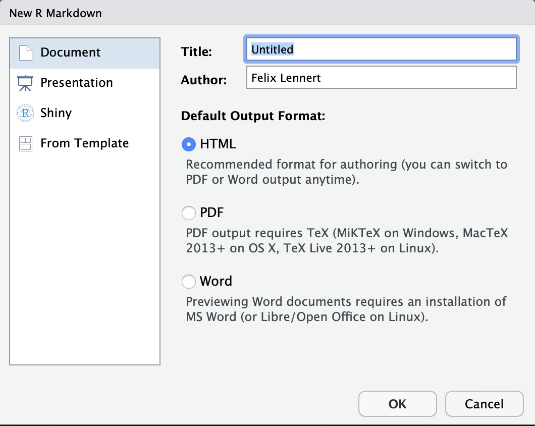
New RMarkdown
Note that you could also do a presentation (with the beamer package), a shiny app, or use templates. We will focus on simple RMarkdown documents2. Here, you can type in a title, the name(s) of the author(s), and choose the default output format. For now you have to choose one, but later you can switch to one of the others whenever you want to.
- HTML is handy for lightweight, quickly knitted files, or if you want to publish it on a website.
- PDF is good if you are experienced with LaTeX and want to further modify it in terms of formatting etc., or simply want to get a more formally looking document (I use it if I need to hand in something that is supposed to be graded). If you want to knit to PDF, you need a running LaTeX version on your machine. If you do not have one, I recommend you to install
tinytex.I linked installation instructions down below. - Word puts out an MS Word document – especially handy if you collaborate with people who are either not experienced in R, like older faculty, or want some parts to be proof-read (remember the Track-Changes function?). Note that you need to have MS Word or LibreOffice installed on your machine.
Did you notice the term “knit”? The logic behind RMarkdown documents is that you edit them in RStudio and then “knit” them. This means that it calls the knitr package. Thereby, all the code you include into the document is executed from scratch. If the code does not work and throws an error, the document will not knit – hence, it needs to be properly written to avoid head-scratching. The knitr package creates a markdown file (suffix: .md). This is then processed by pandoc, a universal document converter. The big advantage of this two-step approach is that it enables a wide range of output formats.
For your first RMarkdown document, choose HTML and click “OK”. Then, you see a new plain-text file which looks like this:
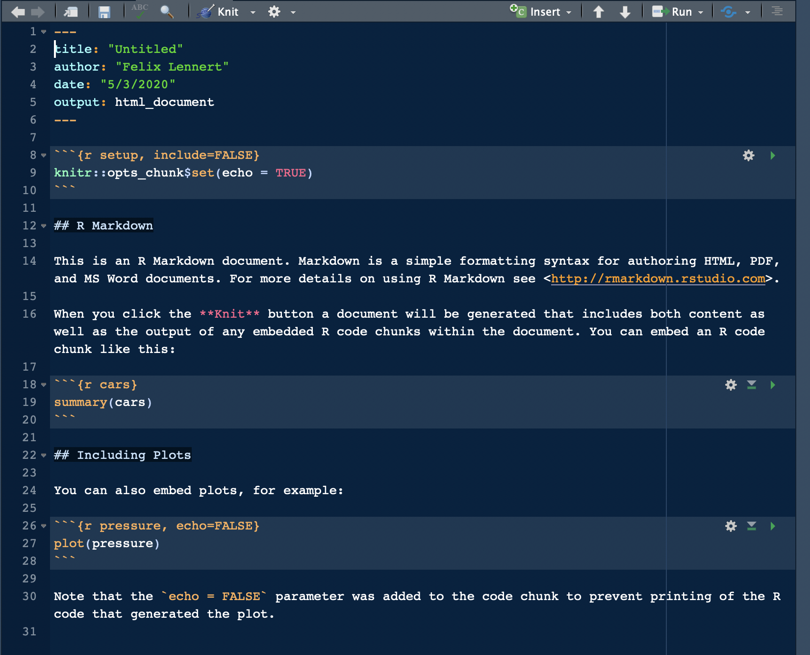
A fresh and clean RMarkdown document
In the top section, surrounded by ---, you can see the so-called YAML header (or YAML metadata, or YAML frontmatter – check out Wikipedia for more information on it). YAML stands for “YAML Ain’t Markup Language” and it is a human-readable data-serialization language. Quick heads-up: indentation matters in your YAML header. This is the metadata of your document. In this minimalistic example, the title, the author, the date, and the desired output are specified (as you specified them when you created the new document). Hence, you can always change them.
After the YAML header, there comes a code chunk. Code chunks start with ```{r} and end with ```. Inside the code chunk, you can write R code which can be executed by either clicking the green “Play” button or by using the same keyboard shortcuts as in scripts. There are several chunk options available: either click on the sprocket or check them out online and include them in the chunk’s header (like this: ```{r include=FALSE}). Beyond that, you can (and should) name your chunks. This makes it easier to find the flawed ones when your document fails to knit. This is done by simply including the name into the title like this: ```{r cars}. Find more on chunk options here.
The double hashes imply that “R Markdown” is a header. In the text, there are examples on how to include links (“<>”), how to make text bold (double asterixes), etc. For more information on how to format plain text in an RMarkdown document, check out the RMarkdown cheatsheet and Reference guide.
1.2.3 Ceci n’est pas un pipe
 For compatibility reasons (the newer pipe requires R 4.1+), we will use the “old” pipe from the
 magrittr package (which is part of the tidyverse) – %>%. The pipe takes its argument on the left and forwards it to the next function, including it there as the first argument unless a . placeholder is provided somewhere. %<>% takes the argument on the left and modifies it at the same time.
library(magrittr)
mean(c(2, 3)) == c(2, 3) %>% mean()
## [1] TRUEmtcars %>% lm(mpg ~ cyl, data = .)##
## Call:
## lm(formula = mpg ~ cyl, data = .)
##
## Coefficients:
## (Intercept) cyl
## 37.885 -2.876# … is the same as…
lm(mpg ~ cyl, data = mtcars)##
## Call:
## lm(formula = mpg ~ cyl, data = mtcars)
##
## Coefficients:
## (Intercept) cyl
## 37.885 -2.876cars <- mtcars
cars %<>% .[[1]] %>% mean()
# … is the same as…
cars <- cars %>% .[[1]] %>% mean()1.2.4 Reading data into R
Data is typically stored in csv-files and can be read in using readr. For “normal,” comma-separated values read_csv("file_path") suffices. Sometimes, a semicolon is used instead of a comma (e.g., in countries that use the commas as a decimal sign). For these files, read_csv2("file_path) is the way to go.
library(tidyverse) # readr is part of the core tidyverse, hence we do not need to load it separately## ── Attaching packages ────────────────────
## ✔ ggplot2 3.4.0 ✔ purrr 1.0.0
## ✔ tibble 3.1.8 ✔ dplyr 1.0.10
## ✔ tidyr 1.2.1 ✔ stringr 1.5.0
## ✔ readr 2.1.3 ✔ forcats 0.5.2
## ── Conflicts ──── tidyverse_conflicts() ──
## ✖ tidyr::extract() masks magrittr::extract()
## ✖ dplyr::filter() masks stats::filter()
## ✖ dplyr::lag() masks stats::lag()
## ✖ purrr::set_names() masks magrittr::set_names()twitter_edgelist <- read_csv("data/edgelist_sen_twitter.csv")#,## Rows: 5657 Columns: 2
## ── Column specification ──────────────────
## Delimiter: ","
## dbl (2): from, to
##
## ℹ Use `spec()` to retrieve the full column specification for this data.
## ℹ Specify the column types or set `show_col_types = FALSE` to quiet this message.# col_types = cols(from = col_character(),
# to = col_character()))1.2.5 Wrangling data with dplyr
The important terms in the dplyr package are mutate(), select(), filter(), summarize() (used with group_by()), and arrange(). pull() can be used to extract a vector. They work with tibbles and data.frames and always take the tibble/data.frame as the first argument (therefore, they work very well with the pipe operator).
# how to create a tibble
horse_tibble <- tibble(
  id = 1:3,
  term = c("horse", "pferd", "cheval"),
  language = c("english", "german", "french")
)

mtcars %>%
  rownames_to_column("model") %>% # add rownames as a column
  select(model, mpg, cyl, hp) %>% # select 4 columns
  arrange(cyl) %>% # arrange them according to number of cylinders
 # filter(cyl %in% c(4, 6)) %>% # only retain values where condition is TRUE
  mutate(model_lowercase = str_to_lower(model)) %>% # change modelnames to lowercase
  group_by(cyl) %>% # change scope, effectively split up tibbles according to group_variable
  summarize(mean_mpg = mean(mpg)) %>% # drop all other columns, collapse rows
  pull(cyl) # pull vector
## [1] 4 6 81.2.6 Visualization
The weapon of choice for visualizing data is ggplot2. (The 2 stands for 2-dimensional graphics.) ggplot2 works with tibbles and the data needs to be in a tidy format. It builds graphics using the “layered grammar of graphics” (Wickham 2010).
library(tidyverse)
library(readxl)

publishers <- read_excel("data/publishers_with_places.xlsx", sheet = "publishers_a-l") %>%
  bind_rows(read_excel("data/publishers_with_places.xlsx", sheet = "publishers_m-z")) %>%
  separate(city, into = c("city", "state"), sep = ",") %>%
  select(publisher, city)

publishers_filtered <- publishers %>%
  group_by(city) %>%
  filter(n() > 5) %>%
  drop_na()
This implies that you start with a base layer – the initial ggplot2 call.
ggplot(data = publishers_filtered)
The initial call produces an empty coordinate system. It can be filled with additional layers.
ggplot(data = publishers_filtered) +
geom_bar(aes(x = city)) 
Unlike the remainder of the tidyverse, ggplot2 uses a + instead of the pipe %>%. If you use the pipe by accident, it will not work and an (informative) error message will appear. There are plenty of geom_.*()s as you probably know already. Each one works a bit differently, but the foundational structure remains the same.
1.2.7 Iteration
We also will work with lists. Lists can contain elements of different lengths (which distinguishes them from tibbles). This makes them especially suitable for web scraping. Other than (atomic) vectors they are not just vectorized since they can contain elements of all different kinds of format.
To iterate over lists, we have the map() family from the purrr package, which applies functions over lists. pluck() extracts elements from the list.
raw_list <- list(first_element = 1:4, 4:6, 10:42)
str(raw_list) # shows you the elements of the list
## List of 3
## $ first_element: int [1:4] 1 2 3 4
## $ : int [1:3] 4 5 6
## $ : int [1:33] 10 11 12 13 14 15 16 17 18 19 ...map(raw_list, mean)## $first_element
## [1] 2.5
##
## [[2]]
## [1] 5
##
## [[3]]
## [1] 26map(raw_list, ~{mean(.x) %>% sqrt()})## $first_element
## [1] 1.581139
##
## [[2]]
## [1] 2.236068
##
## [[3]]
## [1] 5.09902map_dbl(raw_list, mean) # by specifying the type of output, you can reduce the list## first_element
## 2.5 5.0 26.0raw_list %>% pluck(1) == raw_list %>% pluck("first_element")## [1] TRUE TRUE TRUE TRUEThis can also be achieved using a loop. Here, you use an index to loop over objects and do something to their elements. Typically, you create an empty list before and put the new output at the respective new position.
new_list <- vector(mode = "list", length = length(raw_list))
for (i in seq_along(raw_list)){
  new_list[[i]] <- mean(raw_list[[i]])
}
1.2.8 Functions
Another part of R is functions. They require arguments. Then they do something to these arguments. In the end, they return the last call (if it’s not stored in an object). Otherwise, an object can be returned using return() – this is usually unnecessary though.
a_plus_b <- function(a, b){
  a + b
}

a_plus_b(1, 2)
## [1] 3a_plus_b <- function(a, b){
c <- a + b
return(c)
}
a_plus_b(1, 2)## [1] 31.3 Further links
- The R for Data Science book will answer all your questions.
- Yihui Xie published a manual for installing the
tinytexpackage.