Chapter 3 Text Mining
In the final part of this brief introduction to computational techniques for the Social Sciences, I will introduce you to a set of methods that you can use to draw inferences from large text corpora. In specific, this chapter will cover the pre-processing of text, basic (dictionary-based) sentiment analyses, how to weigh terms in a text, supervised classification of documents, and topic modeling. The analyses are performed using “tidy” data principles.
There are a couple of packages around which you can use for text mining, such as quanteda (Benoit et al. 2018) or tm (Feinerer, Hornik, and Meyer 2008), and tidytext (Silge and Robinson 2016) is probably the most recent addition to them. As you could probably tell from its name, tidytext obeys the tidy data principles. “Every observation is a row” translates here to “each token has its own row” – “token” not necessarily relating to a singular term, but also to n-gram, sentence, or paragraph.
In the following, I will demonstrate what text mining using tidy principles can look like in R. The sotu package contains all the so-called “State of the Union” addresses – the president gives them to the congress annually – since 1790.
library(tidyverse)
library(sotu)
sotu_raw <- sotu_meta %>%
  mutate(content = sotu_text)
3.1 Pre-processing: put it into tidy text format
Now that the data is read in, I need to clean it. For this purpose, I take a look at the first entry of the tibble.
sotu_raw %>% slice(1) %>% pull(content) %>% str_sub(1, 500)## [1] "Fellow-Citizens of the Senate and House of Representatives: \n\nI embrace with great satisfaction the opportunity which now presents itself of congratulating you on the present favorable prospects of our public affairs. The recent accession of the important state of North Carolina to the Constitution of the United States (of which official information has been received), the rising credit and respectability of our country, the general and increasing good will toward the government of the Union, an"3.1.1 Cleaning
Nice, that looks pretty clean already. However, I do not need capital letters, line breaks (\n), and punctuation. str_to_lower(), str_replace_all(), and str_squish() from the stringr package (Wickham 2019b) are the right tools for this job. The first one transforms every letter to lowercase, the second one replaces all the occurrences of certain classes with whatever I want it to (a white space in my case), and the final one removes redundant white space (i.e., repeated occurrences of white spaces are reduced to 1).
sotu_clean <- sotu_raw %>%
  mutate(content = str_to_lower(content),
         content = str_replace_all(content, "[^[:alnum:] ]", " "),
         content = str_squish(content))
The next step is to remove stop words – they are not necessary for the sentiment analyses I want to perform first. The stopwords package has a nice list for English.
library(stopwords)
stopwords_vec <- stopwords(language = "en")
#stopwords(language = "de") # the german equivalent
#stopwords_getlanguages() # find the languages that are available
However, it might be easier if I first bring it into the tidy format – every token in a row. Stop words can then be removed by a simple anti_join()
3.1.2 unnest_tokens()
I will focus on the 20th century SOTUs. Here, the dplyr::between() function comes in handy.
sotu_20cent_clean <- sotu_clean %>%
  filter(between(year, 1900, 2000))
Now I can tokenize them:
library(tidytext)

sotu_20cent_tokenized <- sotu_20cent_clean %>%
  unnest_tokens(output = token, input = content)
glimpse(sotu_20cent_tokenized)
## Rows: 917,678
## Columns: 7
## $ X <int> 112, 112, 112, 112, 112, 112, 112, 112, 112, 112, 112, 11…
## $ president <chr> "William McKinley", "William McKinley", "William McKinley…
## $ year <int> 1900, 1900, 1900, 1900, 1900, 1900, 1900, 1900, 1900, 190…
## $ years_active <chr> "1897-1901", "1897-1901", "1897-1901", "1897-1901", "1897…
## $ party <chr> "Republican", "Republican", "Republican", "Republican", "…
## $ sotu_type <chr> "written", "written", "written", "written", "written", "w…
## $ token <chr> "to", "the", "senate", "and", "house", "of", "representat…The new tibble consists of 917,678 rows. Please note that usually you have to put some sort of id column into your original tibble before tokenizing it, e.g., by giving each case – representing a document, or chapter, or whatever – a separate id (e.g., using tibble::rowid_to_column()). This does not apply here, because my original tibble came with a bunch of meta data (president, year, party).
Removing the stop words now is straight-forward:
sotu_20cent_tokenized_nostopwords <- sotu_20cent_tokenized %>%
  filter(!token %in% stopwords_vec)
Another option would have been to anti_join() the tibble which the get_stopwords() function returns. For doing this, the column which contains the singular tokens needs to be called word or a named vector needs to be provided which links the name to word:
sotu_20cent_tokenized_nostopwords <- sotu_20cent_tokenized %>%
  anti_join(get_stopwords(language = "en"), by = c("token" = "word"))
Another thing I forgot to remove are digits. They do not matter for the analyses either:
sotu_20cent_tokenized_nostopwords_nonumbers <- sotu_20cent_tokenized_nostopwords %>%
  filter(!str_detect(token, "[:digit:]"))
Beyond that, I can stem my words using the SnowballC (Porter 2001) package and its function wordStem():
library(SnowballC)
sotu_20cent_tokenized_nostopwords_nonumbers_stemmed <- sotu_20cent_tokenized_nostopwords_nonumbers %>%
  mutate(token = wordStem(token, language = "en"))

#SnowballC::getStemLanguages() # if you want to know the abbreviations for other languages as well
Maybe I should also remove insignificant words, i.e. ones that appear less than 0.5 percent of the time.
sotu_20cent_tokenized_nostopwords_nonumbers_stemmed %>%
  group_by(token) %>%
  filter(n() > nrow(.)/200)
## # A tibble: 30,257 × 7
## # Groups: token [10]
## X president year years_active party sotu_type token
## <int> <chr> <int> <chr> <chr> <chr> <chr>
## 1 112 William McKinley 1900 1897-1901 Republican written congress
## 2 112 William McKinley 1900 1897-1901 Republican written nation
## 3 112 William McKinley 1900 1897-1901 Republican written american
## 4 112 William McKinley 1900 1897-1901 Republican written peopl
## 5 112 William McKinley 1900 1897-1901 Republican written govern
## 6 112 William McKinley 1900 1897-1901 Republican written year
## 7 112 William McKinley 1900 1897-1901 Republican written nation
## 8 112 William McKinley 1900 1897-1901 Republican written congress
## 9 112 William McKinley 1900 1897-1901 Republican written state
## 10 112 William McKinley 1900 1897-1901 Republican written state
## # … with 30,247 more rows3.1.3 In a nutshell
Well, all these things could also be summarized in one nice cleaning pipeline:
sotu_20cent_clean <- sotu_clean %>%
  filter(between(year, 1900, 2000)) %>%
  unnest_tokens(output = token, input = content) %>%
  anti_join(get_stopwords(), by = c("token" = "word")) %>%
  filter(!str_detect(token, "[:digit:]")) %>%
  mutate(token = wordStem(token, language = "en")) %>%
  group_by(token) %>%
  filter(n() > 3)
Now I have created a nice tibble containing the SOTU addresses of the 20th century in a tidy format. This is a great point of departure for subsequent analyses.
3.2 Sentiment Analysis
Sentiment analyses are fairly easy when you have your data in tidy text format. As they basically consist of matching the particular words’ sentiment values to the corpus, this can be done with an inner_join(). tidytext comes with four dictionaries: bing, loughran, afinn, and nrc:
walk(c("bing", "loughran", "afinn", "nrc"), ~get_sentiments(lexicon = .x) %>%
       head() %>%
       print())
## # A tibble: 6 × 2
## word sentiment
## <chr> <chr>
## 1 2-faces negative
## 2 abnormal negative
## 3 abolish negative
## 4 abominable negative
## 5 abominably negative
## 6 abominate negative
## # A tibble: 6 × 2
## word sentiment
## <chr> <chr>
## 1 abandon negative
## 2 abandoned negative
## 3 abandoning negative
## 4 abandonment negative
## 5 abandonments negative
## 6 abandons negative
## # A tibble: 6 × 2
## word value
## <chr> <dbl>
## 1 abandon -2
## 2 abandoned -2
## 3 abandons -2
## 4 abducted -2
## 5 abduction -2
## 6 abductions -2
## # A tibble: 6 × 2
## word sentiment
## <chr> <chr>
## 1 abacus trust
## 2 abandon fear
## 3 abandon negative
## 4 abandon sadness
## 5 abandoned anger
## 6 abandoned fearAs you can see here, the dictionaries are mere tibbles with two columns: “word” and “sentiment”. For easier joining, I should rename my column “token” to word.
library(magrittr)
sotu_20cent_clean %<>% rename(word = token)
The AFINN dictionary is the only one with numeric values. You might have noticed that its words are not stemmed. Hence, I need to do this before I can join it with my tibble. To get the sentiment value per document, I need to average it.
sotu_20cent_afinn <- get_sentiments("afinn") %>%
  mutate(word = wordStem(word, language = "en")) %>%
  distinct(word, .keep_all = TRUE) %>%
  inner_join(sotu_20cent_clean, by = "word") %>%
  group_by(year) %>%
  summarize(sentiment = mean(value))
Thereafter, I can just plot it:
sotu_20cent_afinn %>%
  ggplot() +
  geom_line(aes(x = year, y = sentiment))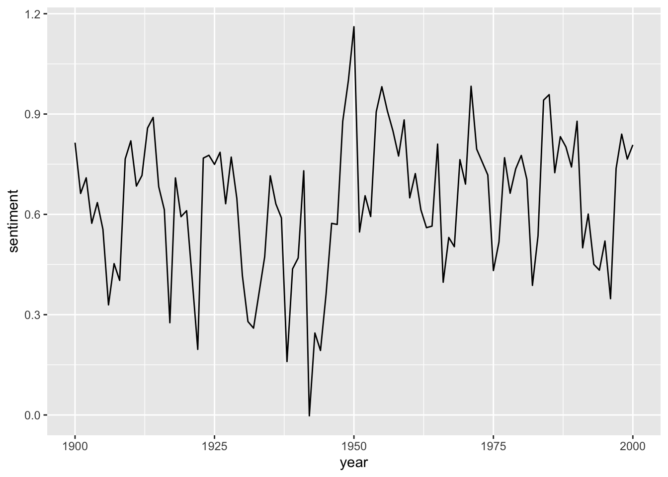
That’s a bit hard to interpret. geom_smooth() might help:
sotu_20cent_afinn %>%
  ggplot() +
  geom_smooth(aes(x = year, y = sentiment))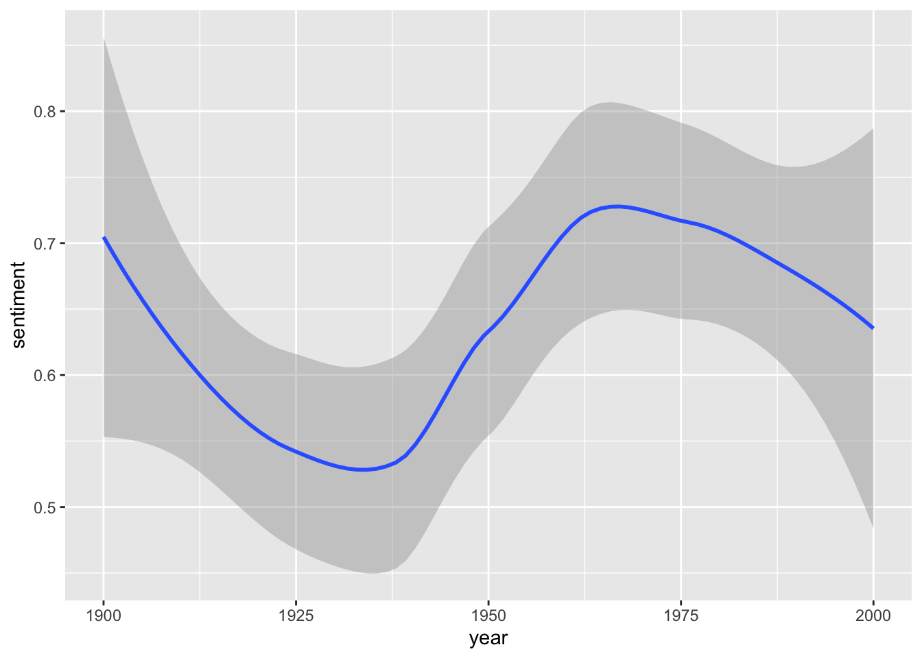
Interesting. When you think of the tone in the SOTU addresses as a proxy measure for the circumstances, the worst phase appears to be during the 1920s and 1930s – might make sense given the then economic circumstances, etc. The maximum was in around the 1960s and since then it has, apparently, remained fairly stable.
3.2.1 Assessing the results
However, we have no idea whether we are capturing some valid signal or not. Let’s look at what drives those classifications the most:
sotu_20cent_contribution <- get_sentiments("afinn") %>%
  mutate(word = wordStem(word, language = "en")) %>%
  inner_join(sotu_20cent_clean)  %>%
  group_by(word) %>%
  summarize(occurences = n(),
            contribution = sum(value))
sotu_20cent_contribution %>%
slice_max(contribution, n = 10) %>%
bind_rows(sotu_20cent_contribution %>% slice_min(contribution, n = 10)) %>%
mutate(word = reorder(word, contribution)) %>%
ggplot(aes(contribution, word, fill = contribution > 0)) +
geom_col(show.legend = FALSE) +
labs(y = NULL)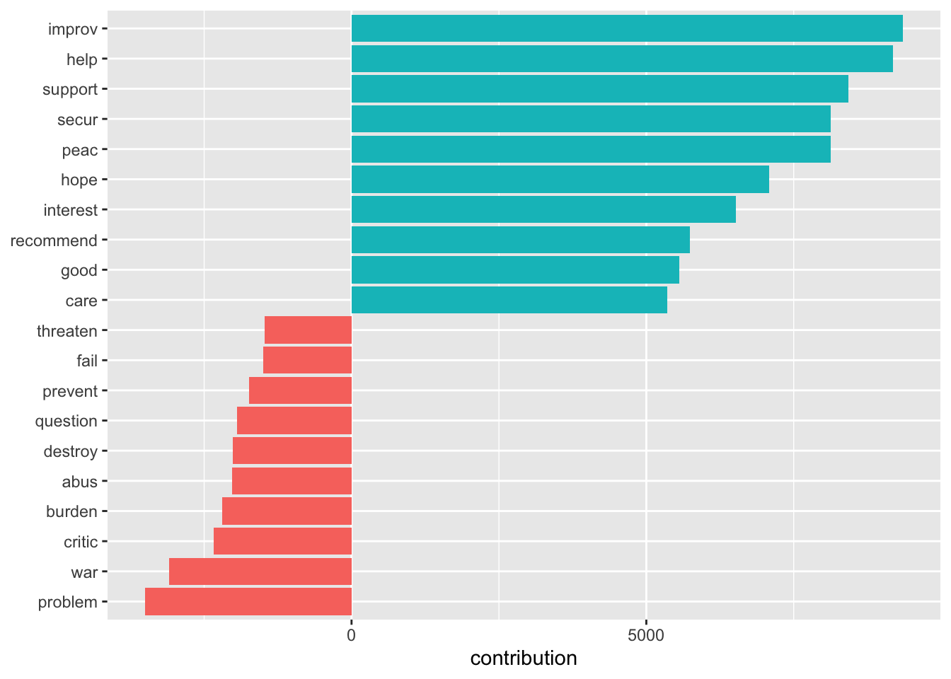
Let’s split this up per decade:
get_sentiments("afinn") %>%
  mutate(word = wordStem(word, language = "en")) %>%
  inner_join(sotu_20cent_clean) %>%
  mutate(decade = ((year - 1900)/10) %>% floor()) %>%
  group_by(decade, word) %>%
  summarize(occurrences = n(),
            contribution = sum(value)) %>%
  slice_max(contribution, n = 5) %>%
  bind_rows(get_sentiments("afinn") %>%
              mutate(word = wordStem(word, language = "en")) %>%
              inner_join(sotu_20cent_clean) %>%
              mutate(decade = ((year - 1900)/10) %>% floor()) %>%
              group_by(decade, word) %>%
              summarize(occurrences = n(),
                        contribution = sum(value)) %>%
              slice_min(contribution, n = 5)) %>%
  mutate(word = reorder_within(word, contribution, decade)) %>%
  ggplot(aes(contribution, word, fill = contribution > 0)) +
  geom_col(show.legend = FALSE) +
  facet_wrap(~decade, ncol = 3, scales = "free") +
  scale_y_reordered()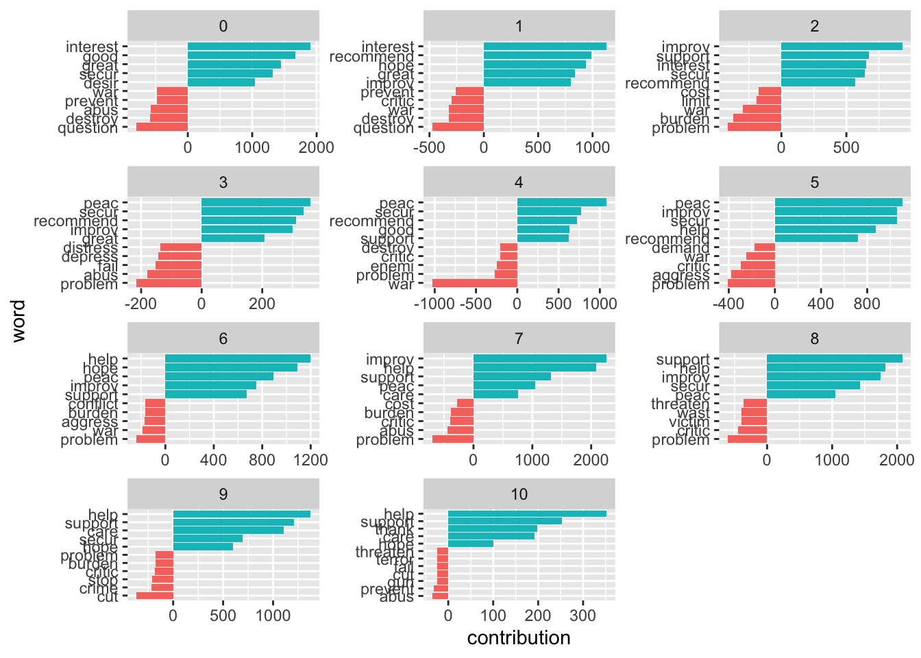
3.2.2 Assessing the quality of the rating
We need to assess the reliability of our classification (would different raters come to the same conclusion; and, if we compare it to a gold standard, how does the classification live up to its standards). One measure we can use here is Krippendorf’s Alpha which is defined as
\[\alpha = \frac{D_o}{D_e}\]
where \(D_{o}\) is the observed disagreement and \(D_{e}\) is the expected disagreement (by chance). The calculation of the measure is far more complicated, but R can easily take care of that – we just need to feed it with proper data. For this example I use a commonly used benchmark data set containing IMDb reviews of movies and whether they’re positive or negative.
imdb_reviews <- read_csv("https://www.dropbox.com/s/qdycmngpw9zwyg1/imdb_reviews.csv?dl=1")

glimpse(imdb_reviews)
## Rows: 25,000
## Columns: 2
## $ text <chr> "Once again Mr. Costner has dragged out a movie for far long…
## $ sentiment <chr> "negative", "negative", "negative", "negative", "negative", …imdb_reviews_afinn <- imdb_reviews %>%
rowid_to_column("doc") %>%
unnest_tokens(token, text) %>%
anti_join(get_stopwords(), by = c("token" = "word")) %>%
mutate(stemmed = wordStem(token)) %>%
inner_join(get_sentiments("afinn") %>% mutate(stemmed = wordStem(word))) %>%
group_by(doc) %>%
summarize(sentiment = mean(value)) %>%
mutate(sentiment_afinn = case_when(sentiment > 0 ~ "positive",
TRUE ~ "negative") %>%
factor(levels = c("positive", "negative")))Now we have two classifications, one “gold standard” from the data and the one obtained through AFINN.
review_coding <- imdb_reviews %>%
  mutate(true_sentiment = sentiment %>%
           factor(levels = c("positive", "negative"))) %>%
  select(-sentiment) %>%
  rowid_to_column("doc") %>%
  left_join(imdb_reviews_afinn %>% select(doc, sentiment_afinn))
First, we can check how often AFINN got it right, the accuracy:
sum(review_coding$true_sentiment == review_coding$sentiment_afinn, na.rm = TRUE)/25000## [1] 0.64712However, accuracy is not a perfect metric because it doesn’t tell you anything about the details. For instance, your classifier might just predict “positive” all of the time. If your gold standard has 50 percent “positive” cases, the accuracy would lie at 0.5. We can address this using the following measures.
For the calculation of Krippendorff’s Alpha, the data must be in a different format: a matrix containing with documents as columns and the respective ratings as rows.
library(irr)
mat <- review_coding %>%
  select(-text) %>%
  as.matrix() %>%
  t()

mat[1:3, 1:5]
## [,1] [,2] [,3] [,4] [,5]
## doc " 1" " 2" " 3" " 4" " 5"
## true_sentiment "negative" "negative" "negative" "negative" "negative"
## sentiment_afinn "positive" "negative" "negative" "positive" "positive"colnames(mat) <- mat[1,]
mat <- mat[2:3,]
mat[1:2, 1:5]## 1 2 3 4 5
## true_sentiment "negative" "negative" "negative" "negative" "negative"
## sentiment_afinn "positive" "negative" "negative" "positive" "positive"kripp.alpha(mat, method = "nominal")## Krippendorff's alpha
##
## Subjects = 25000
## Raters = 2
## alpha = 0.266Good are alpha values of around 0.8 – AFINN missed that one.
Another way to evaluate the quality of classification is through a confusion matrix.
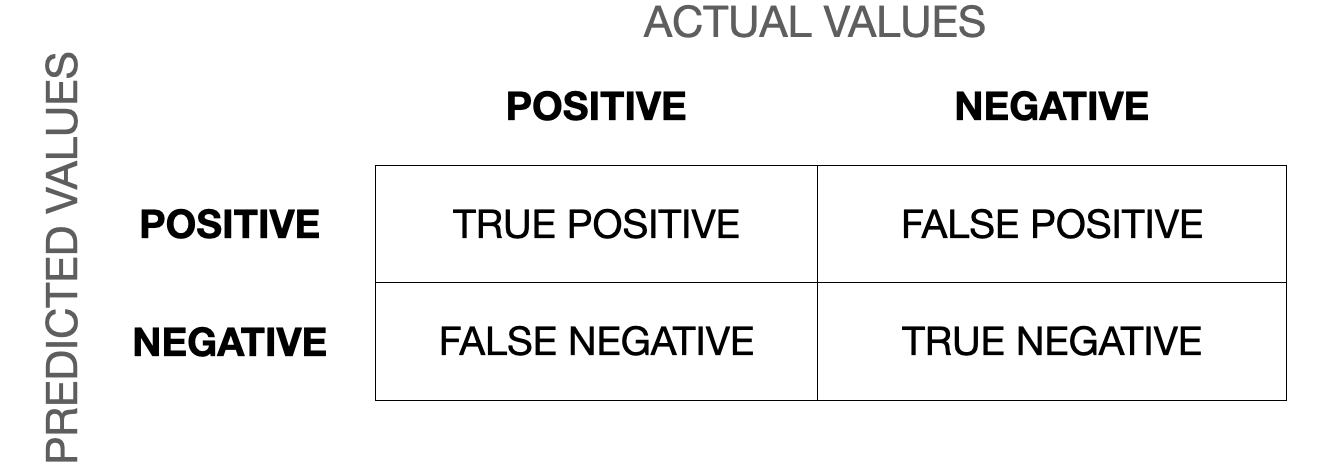
Now we can calculate precision (when it predicts “positive”, how often is it correct), recall/sensitivity (when it is “positive”, how often is this predicted), specificity (when it’s “negative”, how often is it actually negative). The F1-score is the harmonic mean of precision and recall and defined as \(F_1 = \frac{2}{\frac{1}{recall}\times \frac{1}{precision}} = 2\times \frac{precision\times recall}{precision + recall}\) and the most commonly used measure to assess the accuracy of the classification. The closer to 1 it is, the better. You can find a more thorough description of the confusion matrix and the different measures in this blog post.
We can do this in R using the caret package.
library(caret)
confusion_matrix <- confusionMatrix(data = review_coding$sentiment_afinn,
                                    reference = review_coding$true_sentiment,
                                    positive = "positive")
confusion_matrix$byClass
## Sensitivity Specificity Pos Pred Value
## 0.8439750 0.4504721 0.6056500
## Neg Pred Value Precision Recall
## 0.7427441 0.6056500 0.8439750
## F1 Prevalence Detection Rate
## 0.7052216 0.5000000 0.4219875
## Detection Prevalence Balanced Accuracy
## 0.6967515 0.64722363.3 First analyses of content
A common task in the quantitative analysis of text is to determine how documents differ from each other concerning word usage. This is usually achieved by identifying words that are particular for one document but not for another. These words are referred to by Monroe, Colaresi, and Quinn (2008) as fighting words or, by Grimmer, Roberts, and Stewart (2022), discriminating words. To use the techniques that will be presented today, an already existing organization of the documents is assumed.
The most simple approach to determine which words are more correlated to a certain group of documents is by merely counting them and determining their proportion in the document groups. For illustratory purposes, I use fairy tales from H.C. Andersen which are contained in the hcandersenr package.
library(lubridate)

fairytales <- hcandersenr::hcandersen_en %>%
  filter(book %in% c("The princess and the pea",
                     "The little mermaid",
                     "The emperor's new suit"))

fairytales_tidy <- fairytales %>%
  unnest_tokens(output = token, input = text)
3.3.1 Counting words per document
For a first, naive analysis, I can merely count the times the terms appear in the texts. Since the text is in tidytext format, I can do so using means from traditional tidyverse packages. I will then visualize the results with a bar plot.
fairytales_top10 <- fairytales_tidy %>%
  group_by(book) %>%
  count(token) %>%
  slice_max(n, n = 10)
fairytales_top10 %>%
ggplot() +
geom_col(aes(x = n, y = reorder_within(token, n, book))) +
scale_y_reordered() +
labs(y = "token") +
facet_wrap(vars(book), scales = "free") +
theme(strip.text.x = element_blank())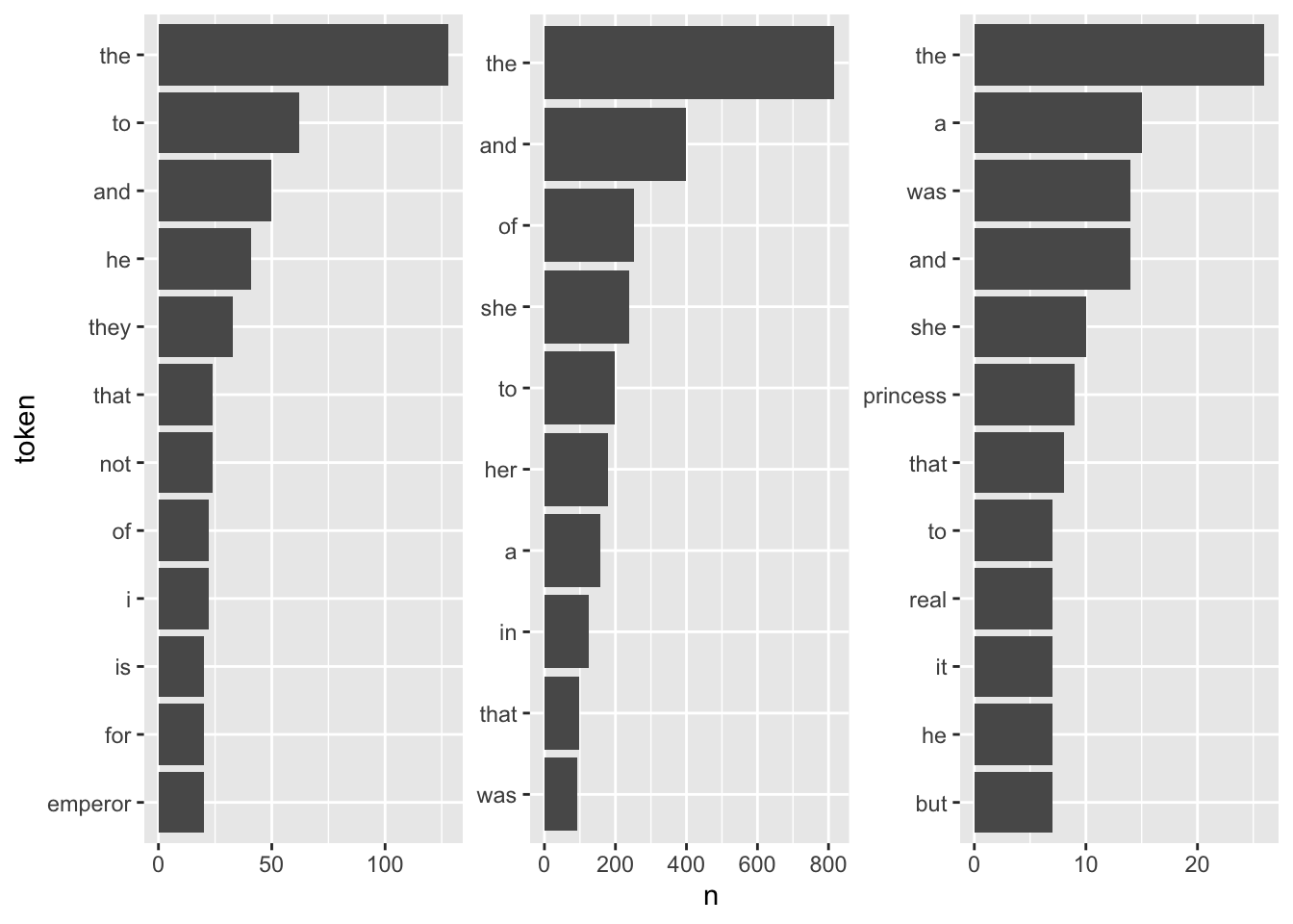
It is quite hard to draw inferences on which plot belongs to which book since the plots are crowded with stopwords. However, there are pre-made stopword lists I can harness to remove some of this “noise” and perhaps catch a bit more signal for determining the books.
library(stopwords)

# get_stopwords()
# stopwords_getsources()
# stopwords_getlanguages(source = "snowball")

fairytales_top10_nostop <- fairytales_tidy %>%
  anti_join(get_stopwords(), by = c("token" = "word")) %>%
  group_by(book) %>%
  count(token) %>%
  slice_max(n, n = 10, with_ties = FALSE)
fairytales_top10_nostop %>%
ggplot() +
geom_col(aes(x = n, y = reorder_within(token, n, book))) +
scale_y_reordered() +
labs(y = "token") +
facet_wrap(vars(book), scales = "free_y") +
scale_x_continuous(breaks = scales::pretty_breaks()) +
theme(strip.text.x = element_blank())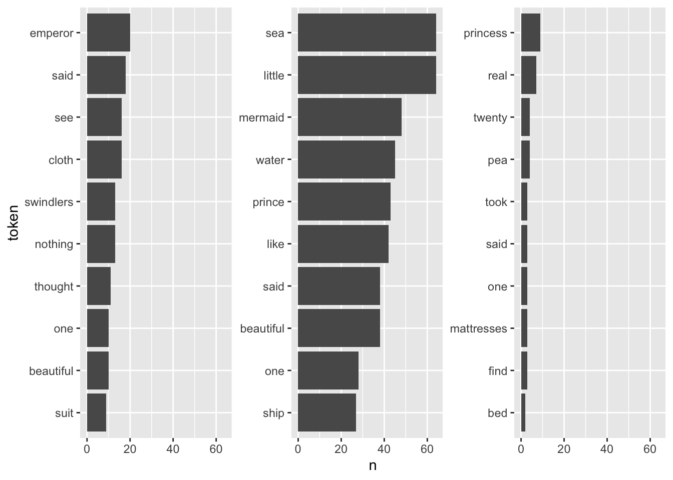
This already looks quite nice, it is quite easy to see which plot belongs to the respective book.
3.3.2 TF-IDF
A better definition of words that are particular to a group of documents is “the ones that appear often in one group but rarely in the other one(s)”. So far, the measure of term frequency only accounts for how often terms are used in the respective document. I can take into account how often it appears in other documents by including the inverse document frequency. The resulting measure is called tf-idf and describes “the frequency of a term adjusted for how rarely it is used.” (Silge and Robinson 2016: 31) If a term is rarely used overall but appears comparably often in a singular document, it might be safe to assume that it plays a bigger role in that document.
The tf-idf of a word in a document is commonly^[Note that multiple implementations exist, for an overview see, for instance, Manning, Raghavan, and Schütze (2008). One implementation is calculated as follows:
\[w_{i,j}=tf_{i,j}\times ln(\frac{N}{df_{i}})\]
–> \(tf_{i,j}\): number of occurrences of term \(i\) in document \(j\)
–> \(df_{i}\): number of documents containing \(i\)
–> \(N\): total number of documents
Note that the \(ln\) is included so that words that appear in all documents – and do therefore not have discriminatory power – will automatically get a value of 0. This is because \(ln(1) = 0\). On the other hand, if a term appears in, say, 4 out of 20 documents, its ln(idf) is \(ln(20/4) = ln(5) = 1.6\).
The tidytext package provides a neat implementation for calculating the tf-idf called bind_tfidf(). It takes as input the columns containing the term, the document, and the document-term counts n.
fairytales_top10_tfidf <- fairytales_tidy %>%
  group_by(book) %>%
  count(token) %>%
  bind_tf_idf(token, book, n) %>%
  slice_max(tf_idf, n = 10)
fairytales_top10_tfidf %>%
ggplot() +
geom_col(aes(x = tf_idf, y = reorder_within(token, tf_idf, book))) +
scale_y_reordered() +
labs(y = "token") +
facet_wrap(vars(book), scales = "free") +
theme(strip.text.x = element_blank(),
axis.title.x = element_blank(),
axis.text.x = element_blank(),
axis.ticks.x = element_blank())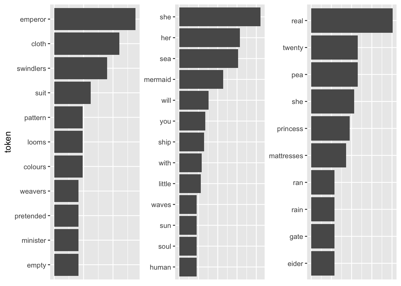
Pretty good already! All the fairytales can be clearly identified. A problem with this representation is that I cannot straightforwardly interpret the x-axis values (they can be removed by uncommenting the last four lines). A way to mitigate this is using odds.
Another shortcoming becomes visible when I take the terms with the highest TF-IDF as compared to all other fairytales.
tfidf_vs_full <- hcandersenr::hcandersen_en %>%
  unnest_tokens(output = token, input = text) %>%
  count(token, book) %>%
  bind_tf_idf(book, token, n) %>%
  filter(book %in% c("The princess and the pea",
                     "The little mermaid",
                     "The emperor's new suit"))

plot_tf_idf <- function(df, group_var){
  df %>%
    group_by({{ group_var }}) %>%
    slice_max(tf_idf, n = 10, with_ties = FALSE) %>%
    ggplot()  +
    geom_col(aes(x = tf_idf, y = reorder_within(token, tf_idf, {{ group_var }}))) +
    scale_y_reordered() +
    labs(y = "token") +
    facet_wrap(vars({{ group_var }}), scales = "free") +
    #theme(strip.text.x = element_blank()) +
    theme(axis.title.x=element_blank(),
          axis.text.x=element_blank(),
          axis.ticks.x=element_blank())
}

plot_tf_idf(tfidf_vs_full, book)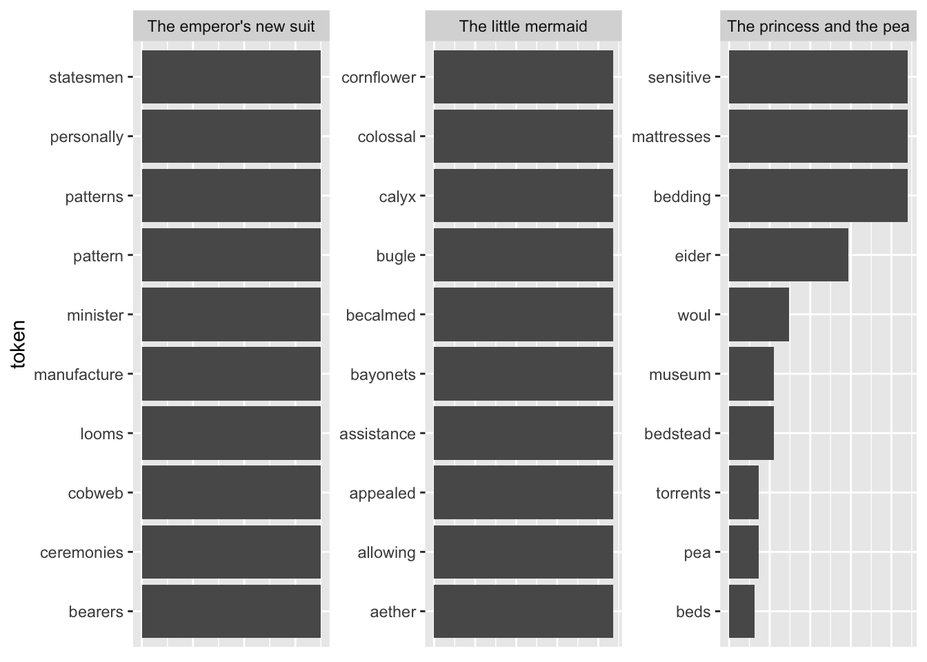
The tokens are far too specific to make any sense. Introducing a lower threshold (i.e., limiting the analysis to terms that appear at least x times in the document) might mitigate that. Yet, this threshold is of course arbitrary.
tfidf_vs_full %>%
  #group_by(token) %>%
  filter(n > 3) %>%
  ungroup() %>%
  plot_tf_idf(book)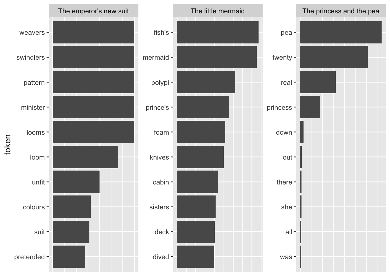
3.4 Machine Learning
In the following subsection, I will introduce you to the supervised and unsupervised classification of text. Supervised means that we will need to “show” the machine a data set that already contains the value or label we want to predict (the “dependent variable”) as well as all the variables that are used to predict the class/value (the independent variables or, in ML lingo, features). In the examples I will showcase, the features are basically the tokens that are contained in a document. Dependent variables are in our examples sentiment or party affiliation.
Unsupervised Learning, on the other hand, implies that the machine is fed with a corpus of different documents and asked to find a new organization for them based on their content. In our examples, we deal with so-called topic models, models that are organizing the documents with regard to their content. Documents which deal with the same set of tokens, i.e., tokens that come from the same topic, are classified as being similar. Moreover, the model learns how different tokens are related to one another. Again, the rationale is that if tokens often appear together in documents, they are probably related to one another and, hence, stem from the same topic.
3.4.1 Supervised Classification
Overall, the process of supervised classification using text in R encompasses the following steps:
- Split data into training and test set
- Pre-processing and featurization
- Training
- Evaluation and tuning (through cross-validation) (… repeat 2.-4. as often as necessary)
- Applying the model to the held-out test set
- Final evaluation
This is mirrored in the workflow() function from the workflows (Vaughan 2022) package. There, you define the pre-processing procedure (add_recipe() – created through the recipe() function from the recipes (Kuhn and Wickham 2022) and/or textrecipes (Hvitfeldt 2022) package(s)), the model specification with add_spec() – taking a model specification as created by the parsnip (Kuhn, Vaughan, and Hvitfeldt 2022) package.
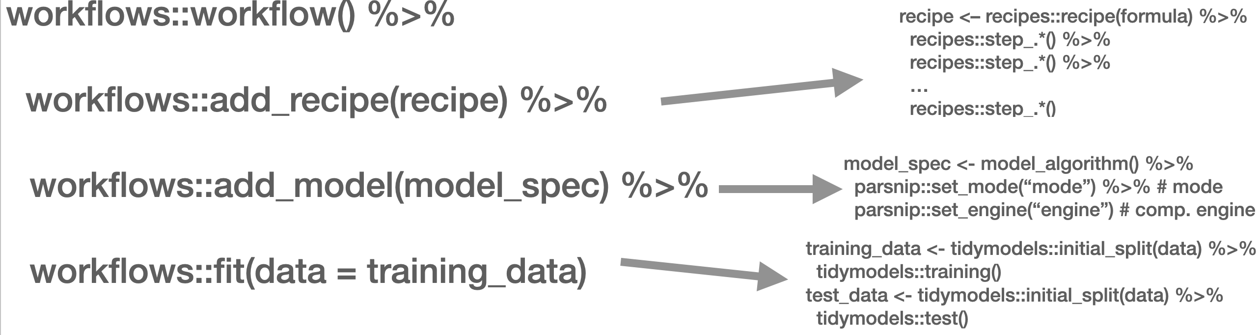
Workflow overview
In the next part, other approaches such as Support Vector Machines (SVM), penalized logistic regression models (penalized here means, loosely speaking, that insignificant predictors which contribute little will be shrunk and ignored – as the text contains many tokens that might not contribute much, those models lend themselves nicely to such tasks), random forest models, or XGBoost will be introduced. Those approaches are not to be explained in-depth, third-party articles will be linked though, but their intuition and the particularities of their implementation will be described. Since we use the tidymodels (Kuhn and Wickham 2020) framework for implementation, trying out different approaches is straightforward. Also, the pre-processing differs: recipes and textrecipes facilitate this task decisively. Third, the evaluation of different classifiers will be described. Finally, the entire workflow will be demonstrated using a Twitter data set.
The first example for today’s session is the IMDb data set. First, we load a whole bunch of packages and the data set.
library(tidymodels)
library(textrecipes)
library(workflows)
library(discrim)
library(glmnet)
library(tidytext)
library(tidyverse)

imdb_full <- read_csv("https://www.dropbox.com/s/0cfr4rkthtfryyp/imdb_reviews.csv?dl=1")

imdb_data <- imdb_full %>% slice_sample(n = 2500)
3.4.1.1 Split the data
The first step is to divide the data into training and test sets using initial_split(). You need to make sure that the test and training set are fairly balanced which is achieved by using strata =. prop = refers to the proportion of observations that makes it into the training set.
split <- initial_split(imdb_data, prop = 0.8, strata = sentiment)

imdb_train <- training(split)
imdb_test <- testing(split)

glimpse(imdb_train)
## Rows: 1,999
## Columns: 2
## $ text <chr> "and nothing else.<br /><br />One of my friends bought the P…
## $ sentiment <chr> "negative", "negative", "negative", "negative", "negative", …imdb_train %>% count(sentiment)## # A tibble: 2 × 2
## sentiment n
## <chr> <int>
## 1 negative 1017
## 2 positive 9823.4.1.2 Pre-processing and featurization
In the tidymodels framework, pre-processing and featurization are performed through so-called recipes. For text data, so-called textrecipes are available.
3.4.1.2.1 textrecipes – basic example
In the initial call, the formula needs to be provided. In our example, we want to predict the sentiment (“positive” or “negative”) using the text in the review. Then, different steps for pre-processing are added. Similar to what you have learned in the prior chapters containing measures based on the bag of words assumption, the first step is usually tokenization, achieved through step_tokenize(). In the end, the features need to be quantified, either through step_tf(), for raw term frequencies, or step_tfidf(), for TF-IDF. In between, various pre-processing steps such as word normalization (i.e., stemming or lemmatization), and removal of rare or common words Hence, a recipe for a very basic model just using raw frequencies and the 1,000 most common words would look as follows:
imdb_basic_recipe <- recipe(sentiment ~ text, data = imdb_train) %>%
  step_tokenize(text) %>% # tokenize text
  step_tokenfilter(text, max_tokens = 1000) %>% # only retain 1000 most common words
  # additional pre-processing steps can be added, see next chapter
  step_tfidf(text) # final step: add term frequencies
In case you want to know what the data set for the classification task looks like, you can prep() and finally bake() the recipe. Note that we need to specify the data set we want to pre-process in the recipe’s manner. In our case, we want to perform the operations on the data specified in the basic_recipe and, hence, need to specify new_data = NULL.
imdb_basic_recipe %>%
  prep() %>%
  bake(new_data = NULL)
## # A tibble: 1,999 × 1,001
## sentiment tfidf_tex…¹ tfidf…² tfidf…³ tfidf…⁴ tfidf…⁵ tfidf…⁶ tfidf…⁷ tfidf…⁸
## <fct> <dbl> <dbl> <dbl> <dbl> <dbl> <dbl> <dbl> <dbl>
## 1 negative 0 0 0 0 0 0 0 0
## 2 negative 0 0 0 0 0 0 0 0
## 3 negative 0 0 0 0 0 0 0 0
## 4 negative 0 0 0 0 0 0 0 0
## 5 negative 0 0 0 0 0 0 0 0
## 6 negative 0 0 0 0 0 0 0.0353 0
## 7 negative 0 0 0 0 0 0 0 0
## 8 negative 0 0 0 0 0 0 0 0
## 9 negative 0 0 0 0 0 0 0 0
## 10 negative 0 0 0 0 0 0 0 0
## # … with 1,989 more rows, 992 more variables: tfidf_text_8 <dbl>,
## # tfidf_text_80 <dbl>, tfidf_text_9 <dbl>, tfidf_text_a <dbl>,
## # tfidf_text_able <dbl>, tfidf_text_about <dbl>, tfidf_text_above <dbl>,
## # tfidf_text_absolutely <dbl>, tfidf_text_across <dbl>, tfidf_text_act <dbl>,
## # tfidf_text_acted <dbl>, tfidf_text_acting <dbl>, tfidf_text_action <dbl>,
## # tfidf_text_actor <dbl>, tfidf_text_actors <dbl>, tfidf_text_actress <dbl>,
## # tfidf_text_actual <dbl>, tfidf_text_actually <dbl>, tfidf_text_add <dbl>, …3.4.1.3 textrecipes – further preprocessing steps
More steps exist. These always follow the same structure: their first two arguments are the recipe (which in practice does not matter, because they are generally used in a “pipeline”) and the variable that is affected (in our example “text” because it is the one to be modified). The rest of the arguments depends on the function. In the following, we will briefly list them and their most important arguments. Find the exhaustive list here,
step_tokenfilter(): filters tokensmax_times =upper threshold for how often a term can appear (removes common words)min_times =lower threshold for how often a term can appear (removes rare words)max_tokens =maximum number of tokens to be retained; will only keep the ones that appear the most often- you should filter before using
step_tforstep_tfidfto limit the number of variables that are created
step_lemma(): allows you to extract the lemma- in case you want to use it, make sure you tokenize via
spacyr(by usingstep_tokenize(text, engine = "spacyr"))
- in case you want to use it, make sure you tokenize via
step_pos_filter(): adds the Part-of-speech tagskeep_tags =character vector that specifies the types of tags to retain (default is “NOUN”, for more details see here)- in case you want to use it, make sure you tokenize via
spacyr(by usingstep_tokenize(text, engine = "spacyr"))
step_stem(): stems tokenscustom_stem =specifies the stemming function. Defaults toSnowballC. Custom functions can be provided.options =can be used to provide arguments (stored as named elements of a list) to the stemming function. E.g.,step_stem(text, custom_stem = "SnowballC", options = list(language = "russian"))
step_stopwords(): removes stopwordssource =alternative stopword lists can be used; potential values are contained instopwords::stopwords_getsources()custom_stopword_source =provide your own stopword listlanguage =specify language of stop word list; potential values can be found instopwords::stopwords_getlanguages()
step_ngram(): takes into account order of terms, provides more contextnum_tokens =number of tokens in n-gram – defaults to 3 – trigramsmin_num_tokens =minimal number of tokens in n-gram –step_ngram(text, num_tokens = 3, min_num_tokens = 1)will return all uni-, bi-, and trigrams.
step_word_embeddings(): use pre-trained embeddings for wordsembeddings(): tibble of pre-trained embeddings
step_normalize(): performs unicode normalization as a preprocessing stepnormalization_form =which Unicode Normalization to use, overview instringi::stri_trans_nfc()
themis::step_upsample()takes care of unbalanced dependent variables (which need to be specified in the call)over_ratio =ratio of desired minority-to-majority frequencies
3.4.1.4 Model specification
Now that the data is ready, the model can be specified. The parsnip package is used for this. It contains a model specification, the type, and the engine. For Naïve Bayes, this would look like the following (note that you will need to install the relevant packages – here: discrim – before using them):
nb_spec <- naive_Bayes() %>% # the initial function, coming from the parsnip package
  set_mode("classification") %>% # classification for discrete values, regression for continuous ones
  set_engine("naivebayes") # needs to be installed
Other model specifications you might deem relevant:
- Logistic regression
lr_spec <- logistic_reg() %>%
  set_engine("glm") %>%
set_mode("classification")- Logistic regression (penalized with Lasso):
lasso_spec <- logistic_reg(mixture = 1) %>%
  set_engine("glm") %>%
set_mode("classification") - SVM (here,
step_normalize(all_predictors())needs to be the last step in the recipe)
svm_spec <- svm_linear() %>%
  set_mode("regression") %>% # can also be "classification"
set_engine("LiblineaR")- Random Forest (with 1000 decision trees):
rf_spec <- rand_forest(trees = 1000) %>%
  set_engine("ranger") %>%
set_mode("regression") # can also be "classification"- xgBoost (with 20 decision trees):
xg_spec <- boost_tree(trees = 20) %>%
  set_engine("xgboost") %>%
  set_mode("regression") # can also be classification
3.4.1.5 Model training – workflows
A workflow can be defined to train the model. It will contain the recipe, hence taking care of the pre-processing, and the model specification. In the end, it can be used to fit the model.
imdb_nb_wf <- workflow() %>%
  add_recipe(imdb_basic_recipe) %>%
  add_model(nb_spec)

imdb_nb_wf
## ══ Workflow ══════════════════════════════
## Preprocessor: Recipe
## Model: naive_Bayes()
##
## ── Preprocessor ──────────────────────────
## 3 Recipe Steps
##
## • step_tokenize()
## • step_tokenfilter()
## • step_tfidf()
##
## ── Model ─────────────────────────────────
## Naive Bayes Model Specification (classification)
##
## Computational engine: naivebayesIt can then be fit using fit().
imdb_nb_basic <- fit(imdb_nb_wf, data = imdb_train)3.4.1.6 Model evaluation
Now that a first model has been trained, its performance can be evaluated. In theory, we have a test set for this. However, the test set is precious and should only be used once we are sure that we have found a good model. Hence, for these intermediary tuning steps, we need to come up with another solution. So-called cross-validation lends itself nicely to this task. The rationale behind it is that chunks from the training set are used as test sets. So, in the case of 10-fold cross-validation, the test set is divided into 10 distinctive chunks of data. Then, 10 models are trained on the respective 9/10 of the training set that is not used for evaluation. Finally, each model is evaluated against the respective held-out “test set” and the performance metrics averaged.

Graph taken from https://scikit-learn.org/stable/modules/cross_validation.html/
First, the folds need to be determined. I set a seed in the beginning to ensure reproducibility.
library(tune)

set.seed(123)
imdb_folds <- vfold_cv(imdb_train)
fit_resamples() trains models on the respective samples.
imdb_nb_resampled <- fit_resamples(
  imdb_nb_wf,
  imdb_folds,
  control = control_resamples(save_pred = TRUE),
  metrics = metric_set(accuracy, recall, precision)
)

#imdb_nb_resampled %>% write_rds("imdb_nb_resampled.rds")
collect_metrics() can be used to evaluate the results.
- Accuracy tells me the share of correct predictions overall
- Precision tells me the number of correct positive predictions
- Recall tells me how many actual positives are predicted properly
In all cases, values close to 1 are better.
collect_predictions() will give you the predicted values.
nb_rs_metrics <- collect_metrics(imdb_nb_resampled)
nb_rs_predictions <- collect_predictions(imdb_nb_resampled)
This can also be used to create the confusion matrix by hand.
confusion_mat <- nb_rs_predictions %>%
  group_by(id) %>%
  mutate(confusion_class = case_when(.pred_class == "positive" & sentiment == "positive" ~ "TP",
                                     .pred_class == "positive" & sentiment == "negative" ~ "FP",
                                     .pred_class == "negative" & sentiment == "negative" ~ "TN",
                                     .pred_class == "negative" & sentiment == "positive" ~ "FN")) %>%
  count(confusion_class) %>%
  ungroup() %>%
  pivot_wider(names_from = confusion_class, values_from = n)
Now you can go back and adapt the pre-processing recipe, fit a new model, or try a different classifier, and evaluate it against the same set of folds. Once you are satisfied, you can proceed to check the workflow on the held-out test data.
3.4.1.7 Hyperparameter tuning
Some models also require the tuning of hyperparameters (for instance, lasso regression). If I wanted to tune these values, I could do so using the tune package. There, the parameter that needs to be tuned gets a placeholder in the model specification. Through variation of the placeholder, the optimal solution can be empirically determined.
So, in the first example, I will try to determine a good penalty value for LASSO regression.
lasso_tune_spec <- logistic_reg(penalty = tune(), mixture = 1) %>%
  set_mode("classification") %>%
  set_engine("glmnet")
I will also play with the numbers of tokens to be included:
imdb_tune_basic_recipe <- recipe(sentiment ~ text, data = imdb_train) %>%
  step_tokenize(text) %>%
  step_tokenfilter(text, max_tokens = tune()) %>%
  step_tf(text)
The dials (Kuhn and Frick 2022) package provides the handy grid_regular() function which chooses suitable values for certain parameters.
lambda_grid <- grid_regular(
  penalty(range = c(-4, 0)),
  max_tokens(range = c(1e3, 2e3)),
  levels = c(penalty = 3, max_tokens = 2)
)
Then, I need to define a new workflow, too.
lasso_tune_wf <- workflow() %>%
  add_recipe(imdb_tune_basic_recipe) %>%
  add_model(lasso_tune_spec)
For the resampling, I can use tune_grid() which will use the workflow, a set of folds (I use the ones I created earlier), and a grid containing the different parameters.
set.seed(123)

tune_lasso_rs <- tune_grid(
  lasso_tune_wf,
  imdb_folds,
  grid = lambda_grid,
  metrics = metric_set(accuracy, sensitivity, specificity)
)
Again, I can access the resulting metrics using collect_metrics():
collect_metrics(tune_lasso_rs)## # A tibble: 18 × 8
## penalty max_tokens .metric .estimator mean n std_err .config
## <dbl> <int> <chr> <chr> <dbl> <int> <dbl> <chr>
## 1 0.0001 1000 accuracy binary 0.771 10 0.0117 Preprocessor1_…
## 2 0.0001 1000 sensitivity binary 0.771 10 0.00996 Preprocessor1_…
## 3 0.0001 1000 specificity binary 0.772 10 0.0160 Preprocessor1_…
## 4 0.01 1000 accuracy binary 0.819 10 0.0115 Preprocessor1_…
## 5 0.01 1000 sensitivity binary 0.802 10 0.0149 Preprocessor1_…
## 6 0.01 1000 specificity binary 0.838 10 0.0158 Preprocessor1_…
## 7 1 1000 accuracy binary 0.509 10 0.0140 Preprocessor1_…
## 8 1 1000 sensitivity binary 1 10 0 Preprocessor1_…
## 9 1 1000 specificity binary 0 10 0 Preprocessor1_…
## 10 0.0001 2000 accuracy binary 0.812 10 0.0114 Preprocessor2_…
## 11 0.0001 2000 sensitivity binary 0.798 10 0.0164 Preprocessor2_…
## 12 0.0001 2000 specificity binary 0.823 10 0.0152 Preprocessor2_…
## 13 0.01 2000 accuracy binary 0.838 10 0.00947 Preprocessor2_…
## 14 0.01 2000 sensitivity binary 0.815 10 0.0114 Preprocessor2_…
## 15 0.01 2000 specificity binary 0.861 10 0.0128 Preprocessor2_…
## 16 1 2000 accuracy binary 0.509 10 0.0140 Preprocessor2_…
## 17 1 2000 sensitivity binary 1 10 0 Preprocessor2_…
## 18 1 2000 specificity binary 0 10 0 Preprocessor2_…autoplot() can be used to visualize them:
autoplot(tune_lasso_rs) +
  labs(
    title = "Lasso model performance across 3 regularization penalties"
  )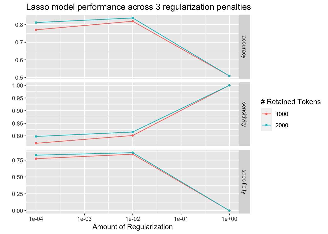
Also, I can use show_best() to look at the best result. Subsequently, select_best() allows me to choose it. In real life, I would choose the best trade-off betIen a model as simple and as good as possible. Using select_by_pct_loss(), I choose the one that performs still more or less on par with the best option (i.e., within 2 percent accuracy) but is considerably simpler. Finally, once I am satisfied with the outcome, I can finalize_workflow() and fit the final model to the test data.
show_best(tune_lasso_rs, "accuracy")## # A tibble: 5 × 8
## penalty max_tokens .metric .estimator mean n std_err .config
## <dbl> <int> <chr> <chr> <dbl> <int> <dbl> <chr>
## 1 0.01 2000 accuracy binary 0.838 10 0.00947 Preprocessor2_Mode…
## 2 0.01 1000 accuracy binary 0.819 10 0.0115 Preprocessor1_Mode…
## 3 0.0001 2000 accuracy binary 0.812 10 0.0114 Preprocessor2_Mode…
## 4 0.0001 1000 accuracy binary 0.771 10 0.0117 Preprocessor1_Mode…
## 5 1 1000 accuracy binary 0.509 10 0.0140 Preprocessor1_Mode…final_lasso_imdb <- finalize_workflow(lasso_tune_wf, select_by_pct_loss(tune_lasso_rs, metric = "accuracy", -penalty))3.4.1.8 Final fit
Now I can finally fit our model to the training data and predict on the test data. last_fit() is the way to go. It takes the workflow and the split (as defined by initial_split()) as parameters.
final_fitted <- last_fit(final_lasso_imdb, split)

collect_metrics(final_fitted)
## # A tibble: 2 × 4
## .metric .estimator .estimate .config
## <chr> <chr> <dbl> <chr>
## 1 accuracy binary 0.806 Preprocessor1_Model1
## 2 roc_auc binary 0.884 Preprocessor1_Model1collect_predictions(final_fitted) %>%
conf_mat(truth = sentiment, estimate = .pred_class) %>%
autoplot(type = "heatmap")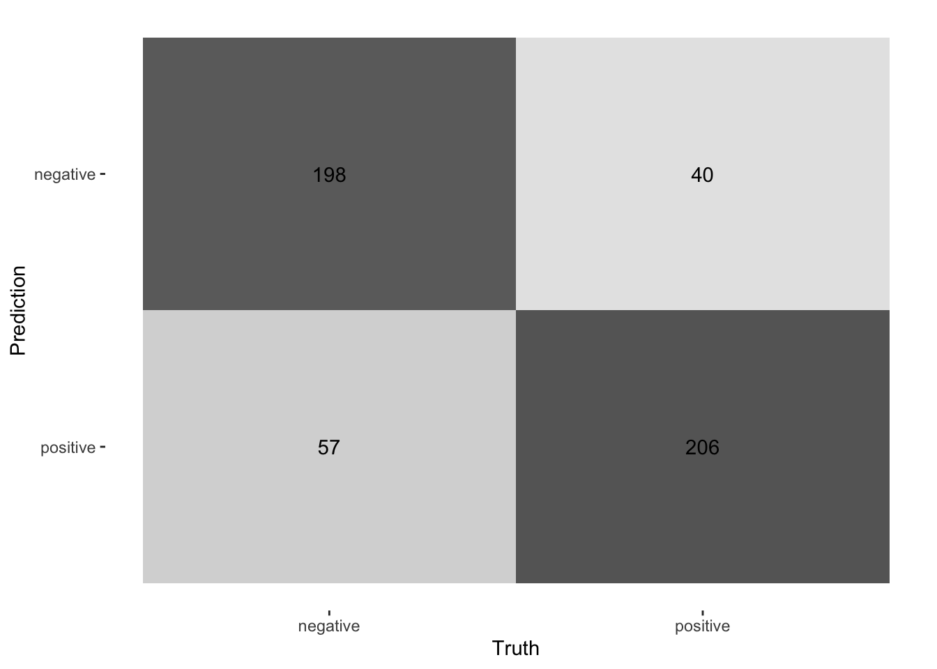
3.4.2 Supervised ML with tidymodels in a nutshell
Here, I give you the condensed version of how you would train a model on a number of documents and predict on a certain test set. To exemplify this, I use Tweets from British MPs from the two largest parties.
First, you take your data and split it into training and test set:
set.seed(1)
timelines_gb <- read_csv("https://www.dropbox.com/s/1lrv3i655u5d7ps/timelines_gb_2022.csv?dl=1")
## Rows: 59444 Columns: 2
## ── Column specification ──────────────────
## Delimiter: ","
## chr (2): party, text
##
## ℹ Use `spec()` to retrieve the full column specification for this data.
## ℹ Specify the column types or set `show_col_types = FALSE` to quiet this message.split_gb <- initial_split(timelines_gb, prop = 0.3, strata = party)
party_tweets_train_gb <- training(split_gb)
party_tweets_test_gb <- testing(split_gb)Second, define your text pre-processing steps. In this case, I want to predict partisanship based on textual content. I tokenize the text, upsample to have balanced classed in terms of party in the training set, and retain only the 1,000 most commonly appearing tokens.
twitter_recipe <- recipe(party ~ text, data = party_tweets_train_gb) %>%
step_tokenize(text) %>% # tokenize text
themis::step_upsample(party) %>%
step_tokenfilter(text, max_tokens = 1000) %>%
step_tfidf(text) Third, the model specification needs to be defined. In this case, I go with a random forest classifier containing 50 decision trees.
rf_spec <- rand_forest(trees = 50) %>%
set_engine("ranger") %>%
set_mode("classification") Finally, the pre-processing “recipe” and the model specification can be summarized in one workflow and the model can be fit to the training data.
twitter_party_rf_workflow <- workflow() %>%
add_recipe(twitter_recipe) %>%
add_model(rf_spec)
party_gb <- twitter_party_rf_workflow %>% fit(data = party_tweets_train_gb)Now I have arrived at a model I can apply to make predictions using augment(). Finally, I can evaluate its accuracy on the test data by taking the share of correctly predicted values.
predictions_gb <- augment(party_gb, party_tweets_test_gb)
mean(predictions_gb$party == predictions_gb$.pred_class)## [1] 0.6989093.4.3 Unsupervised Learning: Topic Models
The two main assumptions of the most commonly used topic model, Latent Dirichlet Allocation (LDA) (Blei, Ng, and Jordan 2003), are as follows:
- Every document is a mixture of topics.
- Every topic is a mixture of words.
Hence, singular documents do not necessarily be distinct in terms of their content. They can be related if they contain the same topics. This is fairly in line with natural language use.
The following graphic depicts a flowchart of text analysis with the tidytext package.
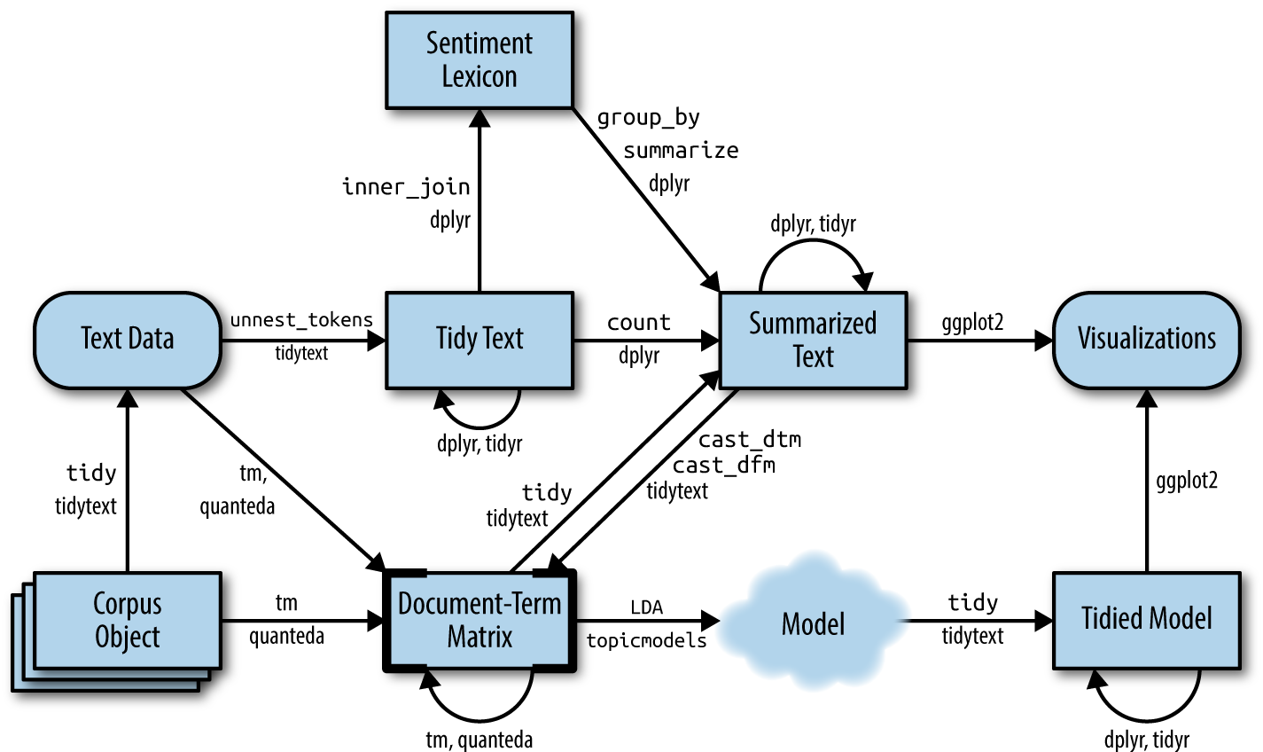
Text analysis flowchart
What becomes evident is that the actual topic modeling will not happen within tidytext. For this, the text needs to be transformed into a document-term-matrix and then passed on to the topicmodels package (Grün et al. 2020), which will take care of the modeling process. Thereafter, the results are turned back into a tidy format, using broom so that they can be visualized using ggplot2.
3.4.3.1 Document-term matrix
To search for the topics which are prevalent in the singular addresses through LDA, we need to transform the tidy tibble into a document-term matrix first. This can be achieved with cast_dtm().
library(sotu)
library(tidytext)
library(SnowballC)
sotu_clean <- sotu_meta %>%
mutate(text = sotu_text %>%
str_replace_all("[,.]", " ")) %>%
filter(between(year, 1900, 2000)) %>%
unnest_tokens(output = token, input = text) %>%
anti_join(get_stopwords(), by = c("token" = "word")) %>%
filter(!str_detect(token, "[:digit:]")) %>%
mutate(token = wordStem(token, language = "en"))
sotu_dtm <- sotu_clean %>%
filter(str_length(token) > 1) %>%
count(year, token) %>%
group_by(token) %>%
filter(n() < 95) %>% # remove tokens that appear in more than 95 documents (i.e., years)
cast_dtm(document = year, term = token, value = n)A DTM contains Documents (rows) and Terms (columns), and specifies how often a term appears in a document.
sotu_dtm %>% as.matrix() %>% .[1:5, 1:5]## Terms
## Docs abandon abat abettor abey abid
## 1900 1 3 1 2 1
## 1901 2 0 0 0 4
## 1902 3 0 0 0 0
## 1903 3 1 0 0 0
## 1904 1 0 0 1 03.4.3.2 Inferring the number of topics
We need to tell the model in advance how many topics we assume to be present within the document. Since we have neither read all the SOTU addresses (if so, we would probably also not have to use the topic model), we cannot make an educated guess on how many topics are in there.
3.4.3.2.1 ldatuning
LDA offers a couple of parameters to tune, but the most crucial one probably is k, the number of topics. One approach might be to just provide it with wild guesses on how many topics might be in there and then try to make sense of them afterward. ldatuning offers a more structured approach to finding the optimal number of k. It trains multiple models with varying ks and compares them with regard to certain performance metrics.
library(ldatuning)determine_k <- FindTopicsNumber(
sotu_dtm,
topics = seq(from = 2, to = 30, by = 1),
metrics = c("Griffiths2004", "CaoJuan2009", "Arun2010", "Deveaud2014"),
method = "Gibbs",
control = list(seed = 77),
mc.cores = 16L,
verbose = TRUE
)
#determine_k %>% write_rds("lda_tuning.rds")Then we can plot the results and determine which maximizes/minimizes the respctive metrics:
FindTopicsNumber_plot(determine_k)## Warning: The `<scale>` argument of `guides()`
## cannot be `FALSE`. Use "none" instead as
## of ggplot2 3.3.4.
## ℹ The deprecated feature was likely used
## in the ldatuning package.
## Please report the issue at
## <]8;;https://github.com/nikita-moor/ldatuning/issueshttps://github.com/nikita-moor/ldatuning/issues]8;;>.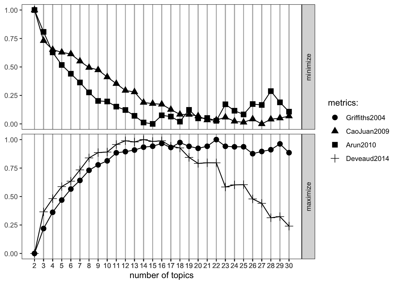
We would go with the 16 topics here, as they seem to maximize the metrics that shall be maximized and minimizes the other ones quite well.
library(topicmodels)
sotu_lda_k16 <- LDA(sotu_dtm, k = 16, control = list(seed = 77))
sotu_lda_k16_tidied <- tidy(sotu_lda_k16)
#write_rds(sotu_lda_k16, "lda_16.rds")Then we can learn a model with this parameter k using the LDA() function.
library(topicmodels)
library(broom)
sotu_lda_k16 <- LDA(sotu_dtm, k = 16, control = list(seed = 77))
sotu_lda_k16_tidied <- tidy(sotu_lda_k16)The tidy() function from the broom package (Robinson 2020) brings the LDA output back into a tidy format. It consists of three columns: the topic, the term, and beta, which is the probability that the term stems from this topic.
sotu_lda_k16_tidied %>% glimpse()## Rows: 171,952
## Columns: 3
## $ topic <int> 1, 2, 3, 4, 5, 6, 7, 8, 9, 10, 11, 12, 13, 14, 15, 16, 1, 2, 3, …
## $ term <chr> "abandon", "abandon", "abandon", "abandon", "abandon", "abandon"…
## $ beta <dbl> 7.884872e-11, 3.156698e-04, 3.691549e-04, 1.782611e-04, 2.385691…Now, we can wrangle it a bit, and then visualize it with ggplot2.
top_terms_k16 <- sotu_lda_k16_tidied %>%
group_by(topic) %>%
slice_max(beta, n = 5, with_ties = FALSE) %>%
ungroup() %>%
arrange(topic, -beta)
top_terms_k16 %>%
mutate(topic = factor(topic),
term = reorder_within(term, beta, topic)) %>%
ggplot(aes(term, beta, fill = topic)) +
geom_bar(stat = "identity", show.legend = FALSE) +
scale_x_reordered() +
facet_wrap(~topic, scales = "free", ncol = 4) +
coord_flip()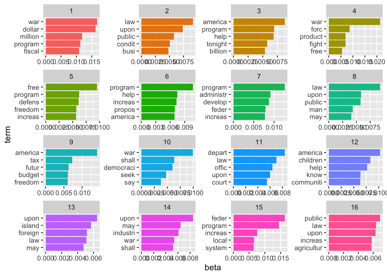
Another thing to assess is document-topic probabilities gamma: which document belongs to which topic. By doing so, you can choose the documents that have the highest probability of belonging to a topic and then read these specifically. This might give you a better understanding of what the different topics might imply.
sotu_lda_k16_document <- tidy(sotu_lda_k16, matrix = "gamma")This shows you the proportion of words in the document which were drawn from the specific topics. In 1990, for instance, many words were drawn from the first topic.
sotu_lda_k16_document %>%
group_by(document) %>%
slice_max(gamma, n = 1) %>%
mutate(gamma = round(gamma, 3))## # A tibble: 99 × 3
## # Groups: document [99]
## document topic gamma
## <chr> <int> <dbl>
## 1 1900 13 1
## 2 1901 2 1
## 3 1902 2 0.997
## 4 1903 8 0.72
## 5 1904 8 0.727
## 6 1905 8 0.998
## 7 1906 8 0.973
## 8 1907 2 0.817
## 9 1908 8 0.613
## 10 1909 11 1
## # … with 89 more rowsAn interesting pattern is that the topics show some time-dependency. This intuitively makes sense, as they might represent some sort of deeper underlying issue.
3.4.3.3 Sense-making
Now, the harder part begins: making sense of the different topics. In LDA, words can exist across topics, making them not perfectly distinguishable. Also, as the number of topics becomes greater, plotting them doesn’t make too much sense anymore.
topic_list <- sotu_lda_k16_tidied %>%
group_by(topic) %>%
group_split() %>%
map_dfc(~.x %>%
slice_max(beta, n = 20, with_ties = FALSE) %>%
arrange(-beta) %>%
select(term)) %>%
set_names(str_c("topic", 1:16, sep = "_"))## New names:
## • `term` -> `term...1`
## • `term` -> `term...2`
## • `term` -> `term...3`
## • `term` -> `term...4`
## • `term` -> `term...5`
## • `term` -> `term...6`
## • `term` -> `term...7`
## • `term` -> `term...8`
## • `term` -> `term...9`
## • `term` -> `term...10`
## • `term` -> `term...11`
## • `term` -> `term...12`
## • `term` -> `term...13`
## • `term` -> `term...14`
## • `term` -> `term...15`
## • `term` -> `term...16`3.4.3.3.1 LDAvis
LDAvis is a handy tool we can use to inspect our model visually. Preprocessing the data is a bit tricky though, therefore we define a quick function first.
library(LDAvis)
prep_lda_output <- function(dtm, lda_output){
doc_length <- dtm %>%
as.matrix() %>%
as_tibble() %>%
rowwise() %>%
summarize(doc_sum = c_across() %>% sum()) %>%
pull(doc_sum)
phi <- posterior(lda_output)$terms %>% as.matrix()
theta <- posterior(lda_output)$topics %>% as.matrix()
vocab <- colnames(dtm)
term_sums <- dtm %>%
as.matrix() %>%
as_tibble() %>%
summarize(across(everything(), ~sum(.x))) %>%
as.matrix()
svd_tsne <- function(x) tsne::tsne(svd(x)$u)
LDAvis::createJSON(phi = phi,
theta = theta,
vocab = vocab,
doc.length = doc_length,
term.frequency = term_sums[1,],
mds.method = svd_tsne
)
}Thereafter, getting the data into format and running the app works as follows.
json_lda <- prep_lda_output(sotu_dtm, sotu_lda_k16)
serVis(json_lda, out.dir = 'vis', open.browser = TRUE)
servr::daemon_stop(1)3.4.3.4 Structural Topic Models
Structural Topic Models offer a framework for incorporating metadata into topic models. In particular, you can have these metadata affect the topical prevalence, i.e., the frequency a certain topic is discussed, which can vary depending on some observed non-textual property of the document. On the other hand, the topical content, i.e., the terms that constitute topics, may vary depending on certain covariates.
Structural Topic Models are implemented in R via a dedicated package. The following overview provides information on the workflow and the functions that facilitate it.
 In the following example, I will use the State of the Union addresses to run you through the process of training and evaluating an STM.
library(stm)## stm v1.3.6 successfully loaded. See ?stm for help.
## Papers, resources, and other materials at structuraltopicmodel.com##
## Attaching package: 'stm'## The following object is masked from 'package:lattice':
##
## cloudsotu_stm <- sotu_meta %>%
mutate(text = sotu_text) %>%
distinct(text, .keep_all = TRUE) %>%
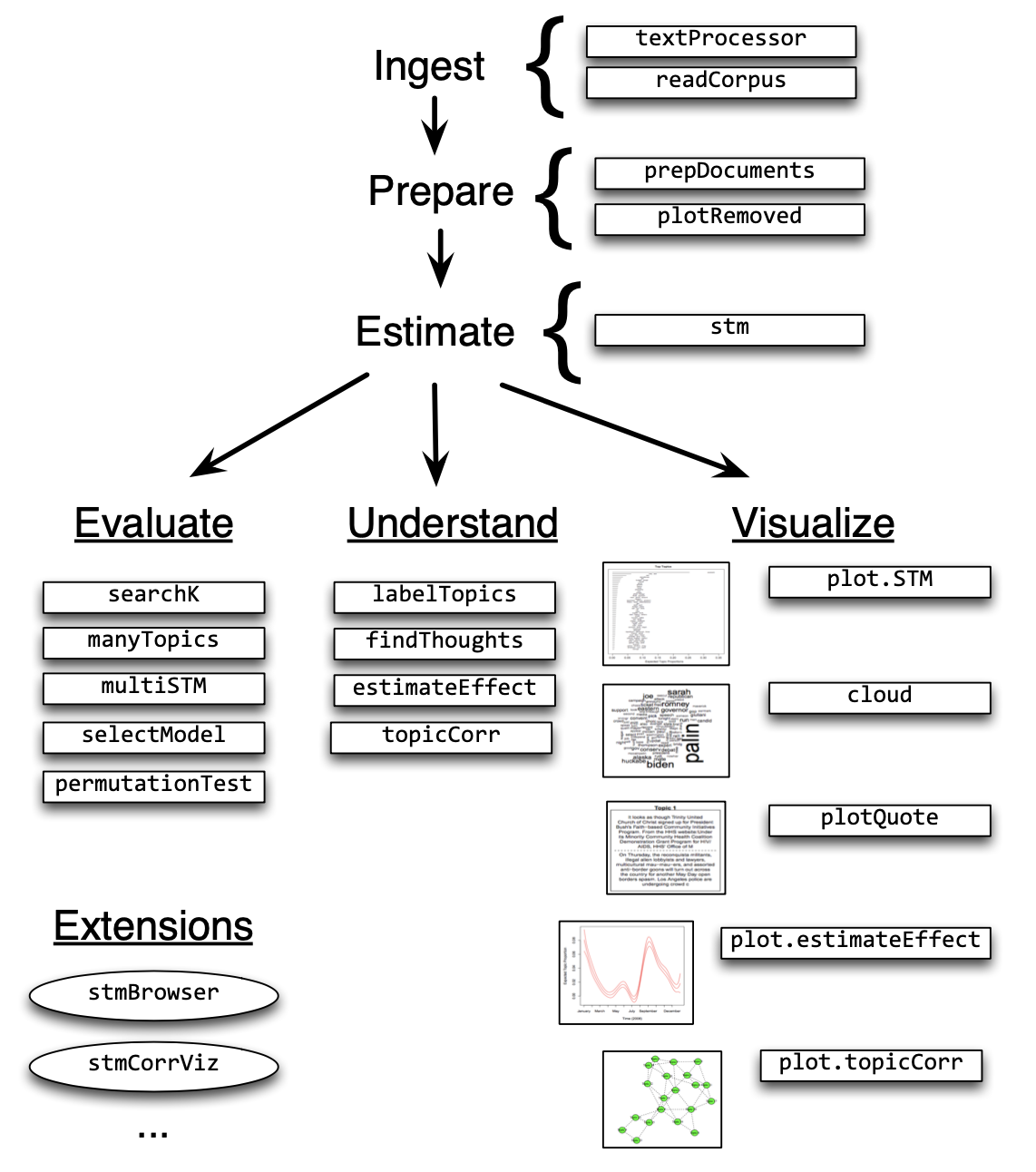
filter(between(year, 1900, 2000))The package requires a particular data structure and has included several functions that help you preprocess your data. textProcessor() takes care of preprocessing the data. It takes as a first argument the text as a character vector as well as the tibble containing the metadata. Its output is a list containing a document list containing word indices and counts, a vocabulary vector containing words associated with these word indices, and a data.frame containing associated metadata. prepDocuments() finally brings the resulting list into a shape that is appropriate for training an STM. It has certain threshold parameters which are geared towards further reducing the vocabulary. lower.thresh = n removes words that are not present in at least n documents, upper.thresh = m removes words that are present in more than m documents. The ramifications of these parameter settings can be explored graphically using the plotRemoved() function.
processed <- textProcessor(sotu_stm$text, metadata = sotu_stm %>% select(-text))## Building corpus...
## Converting to Lower Case...
## Removing punctuation...
## Removing stopwords...
## Removing numbers...
## Stemming...
## Creating Output...plotRemoved(processed$documents, lower.thresh = seq(1, 50, by = 2))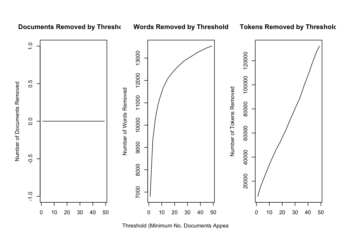
prepped_docs <- prepDocuments(processed$documents, processed$vocab, processed$meta, lower.thresh = 3, upper.thresh = 95)## Removing 9447 of 14346 terms (27061 of 136130 tokens) due to frequency
## Your corpus now has 109 documents, 4899 terms and 109069 tokens.Now that the data is properly preprocessed and prepared, we can estimate the actual model. As mentioned before, covariates can influence topical prevalence as well as their content. I assume topical prevalence to be influenced by the party of the speaker as well as the year the SOTU was held. The latter is assumed to influence the topical prevalence in a non-linear way (SOTU addresses usually deal with acute topics which do not gradually build over time) and is therefore estimated with a spline through the s() function that comes from the stm package. It defaults to a spline with 10 degrees of freedom. Moreover, I assume the content of topics to be influenced by party affiliation. Both prevalence = and content = take their arguments in formula notation.
As determined before, I assume the presence of K = 16 topics (stm also offers the searchK() function to tune this hyperparameter)
sotu_content_fit <- stm(documents = prepped_docs$documents,
vocab = prepped_docs$vocab,
K = 16,
prevalence = ~party + s(year),
content = ~party,
max.em.its = 75,
data = prepped_docs$meta,
init.type = "Spectral",
verbose = FALSE)Let’s look at a summary of the topics and their prevalence. For this, we can use a shiny app developed by Carsten Schwemmer
library(stminsights)
out <- list(documents = prepped_docs$documents,
vocab = prepped_docs$vocab,
meta = prepped_docs$meta)
prepped_docs$meta$party <- as.factor(prepped_docs$meta$party)
prep <- estimateEffect(1:16 ~ party + s(year), sotu_content_fit, meta = prepped_docs$meta, uncertainty = "Global")
map(1:16, ~summary(prep, topics = .x))
save(prepped_docs, sotu_content_fit, prep, out, file = "stm_insights.RData")
run_stminsights()3.4.3.5 Further readings
- Tidy text mining with R.
- A more general introduction by Christopher Bail.
- Supervised Machine Learning for Text Analysis in R by Emil Hvitfeldt and Julia Silge
- More on tidymodels
- Basic descriptions of ML models
- More on prediction with text using tidymodels
- A
shinyintroduction to STM by Thierry Warin
3.5 Exercises
3.5.1 Pre-processing
- Read in the files with Tweets containing the hashtag #musk in 2016 and 2022. Bring them into
tidytextformat (i.e., unnest the tokens).
Solution. Click to expand!
library(tidyverse)
library(tidytext)
musk_tweets_2016 <- read_csv("data/musk_2016.csv") %>%
unnest_tokens(word, text)## Rows: 959 Columns: 5
## ── Column specification ──────────────────
## Delimiter: ","
## chr (1): text
## dbl (2): id, author_id
## lgl (1): possibly_sensitive
## dttm (1): date
##
## ℹ Use `spec()` to retrieve the full column specification for this data.
## ℹ Specify the column types or set `show_col_types = FALSE` to quiet this message.musk_tweets_2022 <- read_csv("data/musk_2022.csv") %>%
unnest_tokens(word, text)## Rows: 10000 Columns: 5
## ── Column specification ──────────────────
## Delimiter: ","
## chr (1): text
## dbl (2): id, author_id
## lgl (1): possibly_sensitive
## dttm (1): date
##
## ℹ Use `spec()` to retrieve the full column specification for this data.
## ℹ Specify the column types or set `show_col_types = FALSE` to quiet this message.- Count the words. Which ones appear the most often in 2016 and 2022 respectively?
- Remove stopwords.
- Stem the words.
How do your results change with every step? Is there more “noise” you would like to have removed – which terms would you remove?
Solution. Click to expand!
musk_tweets_2016 %>%
count(word) %>%
arrange(-n)## # A tibble: 4,078 × 2
## word n
## <chr> <int>
## 1 musk 1045
## 2 https 1038
## 3 t.co 1002
## 4 elon 452
## 5 the 206
## 6 tesla 200
## 7 a 192
## 8 in 169
## 9 rt 169
## 10 to 167
## # … with 4,068 more rowsmusk_tweets_2022 %>%
count(word) %>%
arrange(-n)## # A tibble: 26,746 × 2
## word n
## <chr> <int>
## 1 musk 9400
## 2 https 5578
## 3 t.co 5483
## 4 rt 4920
## 5 elon 3831
## 6 twitter 3435
## 7 a 2329
## 8 tesla 2268
## 9 the 2172
## 10 to 2168
## # … with 26,736 more rows# a
musk_tweets_2016 %>%
anti_join(get_stopwords()) %>%
count(word) %>%
arrange(-n)## Joining, by = "word"## # A tibble: 3,956 × 2
## word n
## <chr> <int>
## 1 musk 1045
## 2 https 1038
## 3 t.co 1002
## 4 elon 452
## 5 tesla 200
## 6 rt 169
## 7 mars 91
## 8 gt 86
## 9 hyperloop 81
## 10 via 77
## # … with 3,946 more rowsmusk_tweets_2022 %>%
anti_join(get_stopwords()) %>%
count(word) %>%
arrange(-n)## Joining, by = "word"## # A tibble: 26,593 × 2
## word n
## <chr> <int>
## 1 musk 9400
## 2 https 5578
## 3 t.co 5483
## 4 rt 4920
## 5 elon 3831
## 6 twitter 3435
## 7 tesla 2268
## 8 de 1701
## 9 elonmusk 1416
## 10 biden 1183
## # … with 26,583 more rows# b
library(SnowballC)
musk_tweets_2016 %>%
anti_join(get_stopwords()) %>%
mutate(word = wordStem(word)) %>%
count(word) %>%
arrange(-n)## Joining, by = "word"## # A tibble: 3,693 × 2
## word n
## <chr> <int>
## 1 musk 1046
## 2 http 1041
## 3 t.co 1002
## 4 elon 452
## 5 tesla 205
## 6 rt 169
## 7 mar 91
## 8 gt 86
## 9 hyperloop 81
## 10 via 77
## # … with 3,683 more rowsmusk_tweets_2022 %>%
anti_join(get_stopwords()) %>%
mutate(word = wordStem(word)) %>%
count(word) %>%
arrange(-n)## Joining, by = "word"## # A tibble: 24,205 × 2
## word n
## <chr> <int>
## 1 musk 9413
## 2 http 5593
## 3 t.co 5483
## 4 rt 4920
## 5 elon 3831
## 6 twitter 3439
## 7 de 2488
## 8 tesla 2276
## 9 elonmusk 1416
## 10 la 1223
## # … with 24,195 more rows3.5.2 Sentiment analysis
- Analyze the SOTU addresses over time using the “bing” dictionary.
- What are the results? Compare them with the “AFINN” analyses from the script.
Solution. Click to expand!
sotu_afinn <- get_sentiments("afinn") %>%
mutate(word = wordStem(word, language = "en")) %>%
inner_join(sotu_clean) %>%
group_by(year) %>%
summarize(sentiment = mean(value))
sotu_bing <- get_sentiments("bing") %>%
mutate(word = wordStem(word, language = "en")) %>%
inner_join(sotu_clean) %>%
mutate(sentiment = case_when(sentiment == "negative" ~ -1,
sentiment == "positive" ~ 1)) %>%
group_by(year) %>%
summarize(sentiment = mean(sentiment))
ggplot(sotu_bing) +
geom_line(aes(x = year, y = sentiment))
sotu_afinn %>%
ggplot() +
geom_line(aes(x = year, y = sentiment))- Which words contribute to them? Again, compare the results with the “AFINN” ones.
Solution. Click to expand!
sotu_afinn_contribution <- get_sentiments("afinn") %>%
mutate(word = wordStem(word, language = "en")) %>%
inner_join(sotu_clean) %>%
group_by(word) %>%
summarize(occurences = n(),
contribution = sum(value)) %>%
mutate(type = "afinn")
sotu_bing_contribution <- get_sentiments("bing") %>%
mutate(word = wordStem(word, language = "en")) %>%
inner_join(sotu_clean) %>%
mutate(sentiment = case_when(sentiment == "negative" ~ -1,
sentiment == "positive" ~ 1)) %>%
group_by(word) %>%
summarize(occurences = n(),
contribution = sum(sentiment)) %>%
mutate(type = "bing")
bind_rows(sotu_afinn_contribution %>% slice_max(contribution, n = 10),
sotu_afinn_contribution %>% slice_min(contribution, n = 10),
sotu_bing_contribution %>% slice_max(contribution, n = 10),
sotu_bing_contribution %>% slice_min(contribution, n = 10)) %>%
mutate(type = as_factor(type),
word = reorder_within(word, contribution, type)) %>%
ggplot(aes(contribution, word, fill = contribution > 0)) +
geom_col(show.legend = FALSE) +
labs(y = NULL) +
scale_y_reordered() +
facet_wrap(~ type, scales = "free_y")- Calculate Intercoder Reliability (i.e., Krippendorff’s Alpha) of both dictionaries.
Solution. Click to expand!
library(caret)
sotus <- sotu_afinn %>% mutate(sentiment_afinn = case_when(sentiment > 0 ~ "positive",
sentiment < 0 ~ "negative",
TRUE ~ NA_character_) %>%
factor(levels = c("positive", "negative"))) %>%
select(-sentiment) %>%
full_join(sotu_bing %>%
mutate(sentiment_bing = case_when(sentiment > 0 ~ "positive",
sentiment < 0 ~ "negative",
TRUE ~ NA_character_) %>%
factor(levels = c("positive", "negative"))) %>%
select(-sentiment),
by = "year") %>%
drop_na()
mat <- matrix(0, nrow = 2, ncol = nrow(sotus))
mat[1, ] <- sotus$sentiment_afinn
mat[2, ] <- sotus$sentiment_bing
mat[1,2:200] <- 2
irr::kripp.alpha(mat, method = "nominal")Krippendorff’s Alpha is 0. This means that it doesn’t really perform better than guessing. This is due to the fact that virtually every SOTU address gets rated “positive” bewertet werden. Krippendorff’s Alpha requires a certain balance though (as you will find in the IMDb data set). More on that in this [ResearchGate discussion] (https://www.researchgate.net/post/Why_is_reliability_so_low_when_percentage_of_agreement_is_high).
- Use “AFINN” and “bing” to classify the IMDb reviews.
- Evaluate the classification quality using
caret::confusionMatrix(). Any differences?
Solution. Click to expand!
imdb_reviews <- read_csv("https://www.dropbox.com/s/qdycmngpw9zwyg1/imdb_reviews.csv?dl=1")
imdb_reviews_afinn <- imdb_reviews %>%
rowid_to_column("doc") %>%
unnest_tokens(token, text) %>%
anti_join(get_stopwords(), by = c("token" = "word")) %>%
mutate(stemmed = wordStem(token)) %>%
inner_join(get_sentiments("afinn") %>% mutate(stemmed = wordStem(word))) %>%
group_by(doc) %>%
summarize(sentiment = mean(value)) %>%
mutate(sentiment_afinn = case_when(sentiment > 0 ~ "positive",
TRUE ~ "negative")) %>%
select(doc, sentiment_afinn)
imdb_reviews_bing <- imdb_reviews %>%
select(-sentiment) %>%
rowid_to_column("doc") %>%
unnest_tokens(token, text) %>%
anti_join(get_stopwords(), by = c("token" = "word")) %>%
mutate(stemmed = wordStem(token)) %>%
inner_join(get_sentiments("bing") %>% mutate(stemmed = wordStem(word))) %>%
mutate(sentiment = case_when(sentiment == "negative" ~ -1,
sentiment == "positive" ~ 1)) %>%
group_by(doc) %>%
summarize(sentiment = mean(sentiment)) %>%
mutate(sentiment_bing = case_when(sentiment > 0 ~ "positive",
TRUE ~ "negative")) %>%
select(doc, sentiment_bing)
reviews <- imdb_reviews %>%
rowid_to_column("doc") %>%
select(-text)
afinn_bing <- inner_join(reviews, imdb_reviews_afinn, by = "doc") %>%
inner_join(imdb_reviews_bing, by = "doc") %>%
mutate(across(starts_with("sentiment"), ~factor(.x, levels = c("positive", "negative"))))
conf_matrix_afinn <- confusionMatrix(data = afinn_bing$sentiment, reference = afinn_bing$sentiment_afinn)
conf_matrix_bing <- confusionMatrix(data = afinn_bing$sentiment, reference = afinn_bing$sentiment_bing)- How could you remodel the “NRC” dictionary to compare its results?
Solution. Click to expand!
get_sentiments("nrc") %>% mutate(sentiment_numeric = case_when(sentiment == "positive" ~ 1,
sentiment == "negative" ~ -1,
TRUE ~ NA_real_)) %>%
drop_na()- Search for the accuracy scores other, more cutting-edge approaches have achieved on the IMDb data set.
Solution. Click to expand!
3.5.3 TF-IDF
(Trigger warning: deals with the U.S. congress discourse on abortion.)
On May 2, 2022, documents from the supreme court were leaked that showed an upcoming decision on one of the major hot-button issues in American politics. Which topic? Can you figure that out from the data? (Hints: perhaps remove hashtags and infrequent words (words with n <= 15)?; use some of the methods outlined above; try to identify the issue)
As we are talking hot-button issue here, how did the language Republican and Democratic House members used differ?
Try to select tweets that are about the issue at hand (i.e., abortion and the leak). Come up with keywords that help you select all relevant tweets. Note that due to the issue and the language concerning it being so partisan, your choice might skew your sample. Focus on tweets posted after the leak. You can check whether you see abortion-related tweets spike using the following code:
tweets_abortion %>% count(date) %>% ggplot() + geom_line(aes(date, n))Group your resulting data according to party affiliation. Are there party-specific language differences you can uncover using the method above?
Solution. Click to expand!
library(tidyverse)
library(rvest)
library(janitor)
library(lubridate)
library(tidytext)
rep_overview <- read_html("https://pressgallery.house.gov/member-data/members-official-twitter-handles") %>%
html_table() %>%
pluck(1)
colnames(rep_overview) <- rep_overview[2, ]
rep_overview <- slice(rep_overview, -1, -2) %>%
janitor::clean_names() %>%
mutate(twitter_handle = str_remove(twitter_handle, "\\@"))
tweets <- read_csv("https://www.dropbox.com/s/c6lssql66rpke5v/congress_tweets_2022.csv?dl=1") %>%
mutate(date_group = case_when(date >= ymd("2022-05-02") ~ "after",
between(date, ymd("2022-04-15"), ymd("2022-05-01")) ~ "before")) %>%
filter(!is.na(date_group)) %>%
left_join(rep_overview %>% select(twitter_handle, party))
tf_idf_min15 <- tweets %>%
#mutate(text = str_remove_all(text, "\\#.* ")) %>%
drop_na(date_group) %>%
unnest_tokens(token, text) %>%
count(token, date_group) %>%
filter(n > 15) %>%
bind_tf_idf(token, date_group, n)
tf_idf_min15 %>% plot_tf_idf(date_group)
keywords <- c("abortion", "prolife", " roe ", "wade ", "roevswade", "baby", "fetus", "womb", "prochoice", "leak")
tweets_abortion <- tweets %>%
filter(str_detect(text, pattern = str_c(keywords, collapse = "|")) &
party %in% c("D", "R"))
tweets_abortion %>%
count(party)
tweets_abortion %>%
count(date) %>%
ggplot() +
geom_line(aes(date, n))
tweets_abortion_new <- tweets %>%
filter(str_detect(text, pattern = str_c(keywords, collapse = "|")) &
date > ymd("2022-05-01") &
party %in% c("D", "R"))
tweets_abortion_new %>%
count(party)
tf_idf_abortion <- tweets_abortion_new %>%
#mutate(text = str_remove_all(text, "\\#.* ")) %>%
filter(party %in% c("D", "R")) %>%
unnest_tokens(token, text) %>%
count(token, party) %>%
bind_tf_idf(token, party, n)
tf_idf_abortion %>% plot_tf_idf(party)3.5.4 Supervised Classification
- Measuring polarization of language through a “fake prediction.” Train the same model that we trained on British MPs earlier on
timelines_us <- read_csv("https://www.dropbox.com/s/dpu5m3xqz4u4nv7/tweets_house_rep_party.csv?dl=1"). First, split the new data into training and test set (prop = 0.3should suffice, make sure that you setstrata = party). Train the model using the same workflow but new training data that predicts partisanship based on the Tweets’ text. Predict on the test set and compare the models’ accuracy.
timelines_gb <- read_csv("https://www.dropbox.com/s/1lrv3i655u5d7ps/timelines_gb_2022.csv?dl=1")
timelines_us <- read_csv("https://www.dropbox.com/s/iglayccyevgvume/timelines_us.csv?dl=1")Solution. Click to expand!
set.seed(1)
split_gb <- initial_split(timelines_gb, prop = 0.3, strata = party)
party_tweets_train_gb <- training(split_gb)
party_tweets_test_gb <- testing(split_gb)
split_us <- initial_split(timelines_us, prop = 0.3, strata = party)
party_tweets_train_us <- training(split_us)
party_tweets_test_us <- testing(split_us)
twitter_recipe <- recipe(party ~ text, data = party_tweets_train_gb) %>%
  step_tokenize(text) %>% # tokenize text
  themis::step_upsample(party) %>%
  step_tokenfilter(text, max_tokens = 1000) %>%
  step_tfidf(text)
rf_spec <- rand_forest(trees = 50) %>%
  set_engine("ranger") %>%
  set_mode("classification")
twitter_party_rf_workflow <- workflow() %>%
  add_recipe(twitter_recipe) %>%
  add_model(rf_spec)

party_gb <- twitter_party_rf_workflow %>% fit(data = party_tweets_train_gb)
party_us <- twitter_party_rf_workflow %>% fit(data = party_tweets_train_us)
predictions_gb <- augment(party_gb, party_tweets_test_gb)
mean(predictions_gb$party == predictions_gb$.pred_class)
predictions_us <- augment(party_us, party_tweets_test_us)
mean(predictions_us$party == predictions_us$.pred_class)- Extract Tweets from U.S. timelines that are about abortion by using a keyword-based sampling approach (
keywords <- c("abortion", "prolife", " roe ", " wade ", "roevswade", "baby", "fetus", "womb", "prochoice", "leak"),timelines_us_abortion <- timelines_us %>% filter(str_detect(text, keywords %>% str_c(collapse = "|")))). Perform the same prediction task (but now withinitial_split(prop = 0.8)). How does the accuracy change?
Solution. Click to expand!
keywords <- c("abortion", "prolife", " roe ", " wade ", "roevswade", "baby", "fetus", "womb", "prochoice", "leak")
timelines_us_abortion <- timelines_us %>% filter(str_detect(text, keywords %>% str_c(collapse = "|")))
split_us_abortion <- initial_split(timelines_us_abortion, prop = 0.8, strata = party)
abortion_tweets_train_us <- training(split_us_abortion)
abortion_tweets_test_us <- testing(split_us_abortion)
abortion_us <- twitter_party_rf_workflow %>% fit(data = abortion_tweets_train_us)
predictions_abortion_us <- augment(abortion_us, abortion_tweets_test_us)
mean(predictions_abortion_us$party == predictions_abortion_us$.pred_class)3.5.5 Topic Models
- Check out
LDAvisand how it orders the topics. Try to make some sense of how they are related etc.
Solution. Click to expand!
json_lda <- prep_lda_output(sotu_dtm, sotu_lda_k16)

serVis(json_lda, out.dir = 'vis', open.browser = TRUE)

servr::daemon_stop(1)- Do the same thing for
stminsights. The trained stm model can be downloadedsotu_stm <- read_rds("https://www.dropbox.com/s/65bukmm42byq0dy/sotu_stm_k16.rds?dl=1").
Solution. Click to expand!
library(sotu)
library(tidytext)
library(SnowballC)
library(stminsights)
sotu_clean <- sotu_meta %>%
mutate(text = sotu_text %>%
str_replace_all("[,.]", " ")) %>%
filter(between(year, 1900, 2000)) %>%
unnest_tokens(output = token, input = text) %>%
anti_join(get_stopwords(), by = c("token" = "word")) %>%
filter(!str_detect(token, "[:digit:]")) %>%
mutate(token = wordStem(token, language = "en"))
sotu_dtm <- sotu_clean %>%
filter(str_length(token) > 1) %>%
count(year, token) %>%
#filter(between(year, 1900, 2000)) %>%
group_by(token) %>%
filter(n() < 95) %>%
cast_dtm(document = year, term = token, value = n)
sotu_stm <- sotu_meta %>%
  mutate(text = sotu_text) %>%
  distinct(text, .keep_all = TRUE) %>%
  filter(between(year, 1900, 2000))
processed <- textProcessor(sotu_stm$text, metadata = sotu_stm %>% select(-text))
#, custompunctuation = "-")
#?textProcessor() # check out the different arguments
#?prepDocuments()
plotRemoved(processed$documents, lower.thresh = seq(1, 50, by = 2))
prepped_docs <- prepDocuments(processed$documents, processed$vocab, processed$meta, lower.thresh = 3, upper.thresh = 80)
prepped_docs$meta$party <- as.factor(prepped_docs$meta$party)
prep <- estimateEffect(1:16 ~ party + s(year), sotu_content_fit, meta = prepped_docs$meta, uncertainty = "Global")
map(1:16, ~summary(prep, topics = .x))
save(prepped_docs, sotu_stm, prep, file = "stm_insights.RData")
run_stminsights()