12 Polling
A word of warning before we begin. This chapter is going to be heavier on math and terminology and less concerned with coding. Sometimes things are really easy to calculate in R, but a little more complex to understand. So we’ll put the emphasis where it is needed when talking about something that is often publicized and discussed in polling. But polling also gives us an opportunity to talk about a few valuable statistical concepts: standard errors, margin of error, and confidence intervals.
12.1 Concepts
Ever wonder how news stations are able to declare the winner of an election before 99% of the actual votes are counted? Or what goes into predicting the winner of an election before any of the votes or counted? Or how a pollster can report that 72% of Americans think social media companies have too much power, despite only talking to a tiny fraction of Americans?
Part of the answer to that question relies on the information in the chapter on Samples, but its also dependent on something called the Central Limit Theorem. We’ll talk about both first, before we dive into the math of how to calculate the results of a poll.
12.1.1 Representative
Back in Chapter 7 we discussed probability samples The reason one would use a probability, as opposed to a non-probability sample, is if they want to be able to assess something about a population. A sample is a subset of the population, and in order for the sample to represent the population they have to similar. IN that chapter we saw how dangerous and misleading it can be to project our findings froma sample onto the population if they aren’t similar. The literay Digest poll had a very large sample, but it was dissimilar from the average voter in 1932, so their results were a poor predictor of how the vote went.
There is a huge difference between reporting that 62% of respondents support reducing prision populations, and 62% of Americans support reducing prision populations. The first statement can be factually true, no matter who you talk to (assuming that 62% of them really did say that). The second statement, where you infere from your sample to the population, is dependent on your sample being representative of the population. But how do we know that just because 62% of a representative sample said something, Americans think a certain way?
We can make that leap based on the central limit theorem. The central limit theorem states that if we take repeated random representative samples from a population, over time the means of those samples will conform to a normal distribution. A little more explanation can help make what that means more clear, let me demonstrate.
Let’s say we’re planning a company picnic and are going to buy ice cream, and want to ensure that we have the correct amount of vanilla and chocolate for everyone. We don’t have time to ask everyone at the company their preference, so we’re just going to ask a random sample of people what their favorite ice cream is. We have 100 employees at the company, but we only have time to get the opinions of 20. And since we’re living in a simplified world for the sake of this example, let’s say the only ice creams are vanilla and chocolate.
What do the first 20 people we ask say?
| chocolate | vanilla |
|---|---|
| 12 | 8 |
Interesting okay, but what would have happened if we’d reshuffled everyone and taken a different random sample?
| chocolate | vanilla |
|---|---|
| 7 | 13 |
And what if we’d done that again?
| chocolate | vanilla |
|---|---|
| 13 | 7 |
Similar, but not exactly the same each time. They come back different, but not entirely dissimilar. One sample doesn’t show that no one likes vanilla and then the next that no one likes chocolate. They all have variability because we’re asking different people, but they sort of cluster around different totals.
What if we did that exercise 1000 times, taking different random samples of 20 people? Let’s look at the total number of votes for vanilla below. And just to be clear, anyone that doesn’t vote for vanilla is then voting for chocolate, so we can see both how many people voted for vanilla and chocolate by just plotting one of the two flavors.
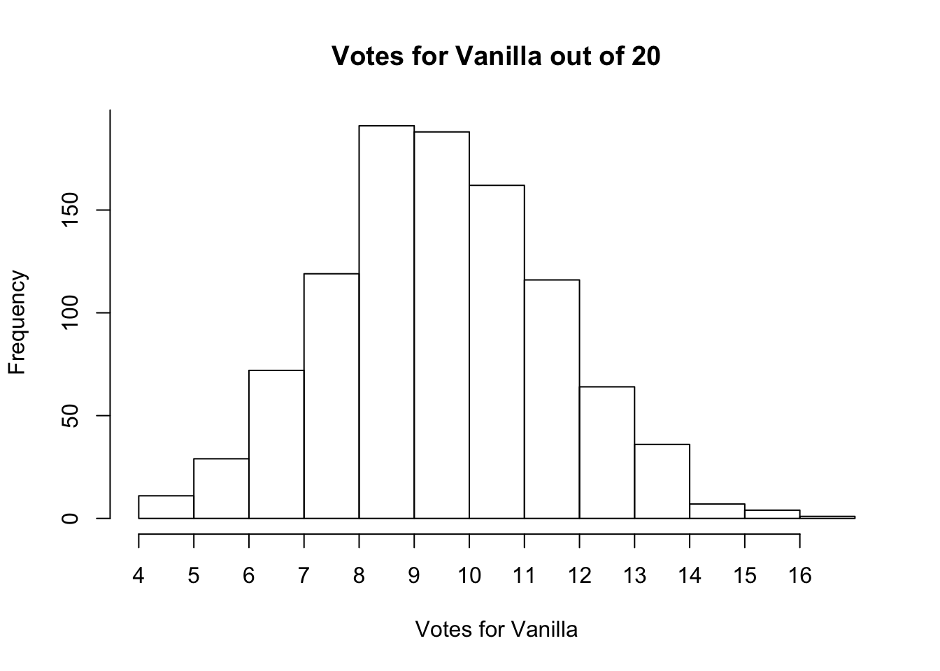
We didn’t identify the exact proportion of people that liked vanilla vs chocolate ice cream with any one sample. The multiple samples we took gave a range of responses, and we can expect that they cluster around the true proportion of votes for each.
This is again driven by the central limit theorem. The central limit theorem states that the mean from a random sample will fall near the mean of the population. It says a lot more than that, but that’s what we tried to demonstrate above. If you take a random sample of employees, the number that will say vanilla vs chocolate will be useful for knowing how many of the population like vanilla and chocolate.
And in fact, the central limit theorem tells us something even more specific about the value we get from each sample. The central limit theorem tells us that the means for samples will form a normal distribution around the population mean. Some will be a little above the population mean, some will be a little the population mean, but they’ll form a predictable shape around it.
We met a normal distribution back in Chapter 10. What’s important about a normal distribution? Well the data forms around the mean evenly, with an equal proportion above and below the mean. But the coolest feature (and I do mean cool) is that the data follows the 68-95-99.7 rule, whereby 68% of the data falls within 1 standard deviation of the mean, 95% falls within 2 standard deviations of the mean, and 99.7 of the data falls within 3 standard deviations of the mean.

Maybe you’re not convinced that’s cool, but trust me it’s about the coolest thing in the world of statistics (IMHO). Why is that helpful? It means that as we showed above, samples taken from a population will generally be close to the population mean, and we actually know the probability of how far they will be from the mean.
If we take a random sample, we can expect that there is a 68% chance it will fall within 1 standard deviation of the mean. That means when we do a sample of ice creams and find that 11 people say vanilla and 9 say chocolate, we can be be confident that result falls with a few standard deviations of the population mean. That’s why taking samples allows us to extrapolate from small amounts of data to an entire population, because the central limit theorem tells us it is highly unlikely the means for our sample will differ significantly from the population.
We took 1000 sample above, and in none of them did 0 people like vanilla or chocolate. The counts were much more likely to be towards the middle of the distribution, with people being equally likely to say vanilla and chocolate. If we took only one sample, and if we were actually planning this party we would only take one sample, we might not know the exact proportion but we’d at least know that there are people that like chocolate and people that like vanilla, so we should be sure to bring both.
That’s similar to what happens during a campaign when pollsters ask people whether they prefer Candidate A or Candidate B. If they take a representative sample, we can expect that the share of people in the sample that say Candidate A is at least somewhat close to the share of people in the population that prefer Candidate A. We can’t be sure that the percentage is exactly correct, just like how in our different samples we didn’t know the exact share of people that like vanilla vs chocolate. But we know that the mean for the sample will generally be close to the population.
Close is an operative word though. We know it should be close, but we can’t be sure that it’s exactly correct Thus, with any survey we acknowledge this by also how precise our results are.
12.1.2 Standard Errors
Since we’re talking polling, let’s meet our candidates for this example
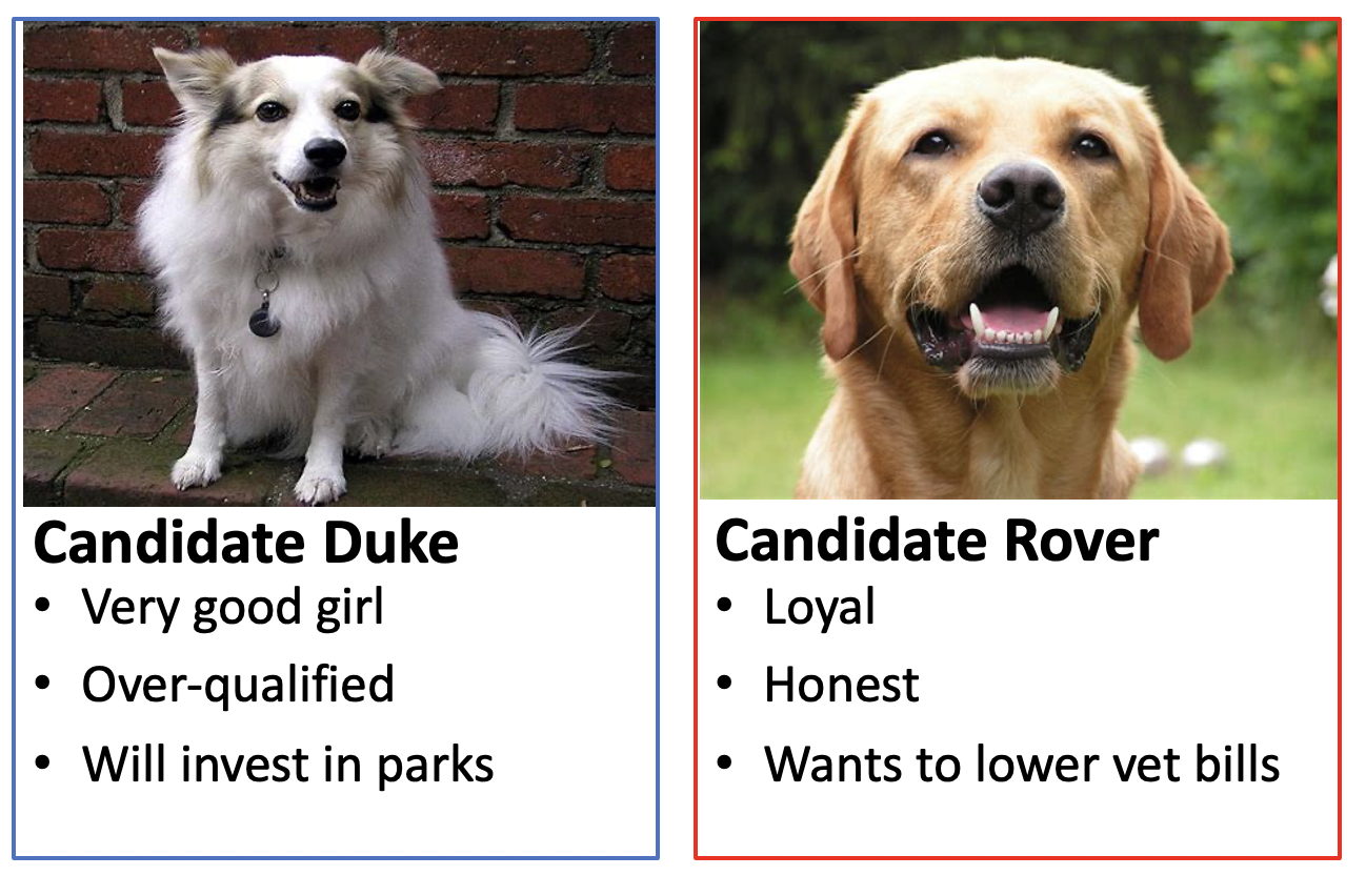
It’s election night, and you’re working for a TV station that is anxious to be the first to declare a winner between Rover and Duke. You conduct an exit poll, which is typically done by asking a represenative sample of people whom they voted for as they leave the polls, and your sample of 1000 people shows that 523 voted for Duke and 477 voted for Rover. You expect 500,000 total votes. Based on the sample you collected is that enough evidence to declare that Duke will win, and how much confidence do you have?
We can first calculate the sample mean. Votes for Duke or Rover are both categorical, but if we give one candidate a value of 1 and the other the value of 0, we can make the data numeric and discrete. If we make all votes for Duke 1, the sample mean becomes .523 or 52.3%, representing how much of the sample voted for that candidate. We could reverse that and give goves for Rover a value of 1, and the sample mean would be .477 or 47.7%, but let’s use Duke for this example.
In order to understand the accuracy of our estimate of the sample mean we can calculate the standard error. Standard error shouldn’t be confused with standard deviation, but they are somewhat similar. While the standard deviation measures the variation or spread of data, the standard error assesses the accuracy of our estimate from a sample.
It is an absolute fact that 52.3% of the sample we collected from the exit poll voted for Duke. What we’re concerned with is how representative we expect that number, 52.3%, to be of the population and how much confidence we can put behind it.
In order to calculate the standard error we need two things: the standard deviation and the sample size. The standard deviation, as we described it in the chapter on descriptive statistics, measures how spread out our data is. The sample size is useful because we can put greater confidence in larger samples than smaller ones. As we learned from the Literary Digest poll, large samples aren’t necessarily better, but a small sample has greater chance for error. The more people we include, the better our chances of odd results sort of evening out.
Let me demonstrate that below. Let’s imagine we have some data with a mean of 100 and a standard deviation of 5. Those are the characteristics of the population. Let’s take different size samples from that population and see how dispersed the data is.
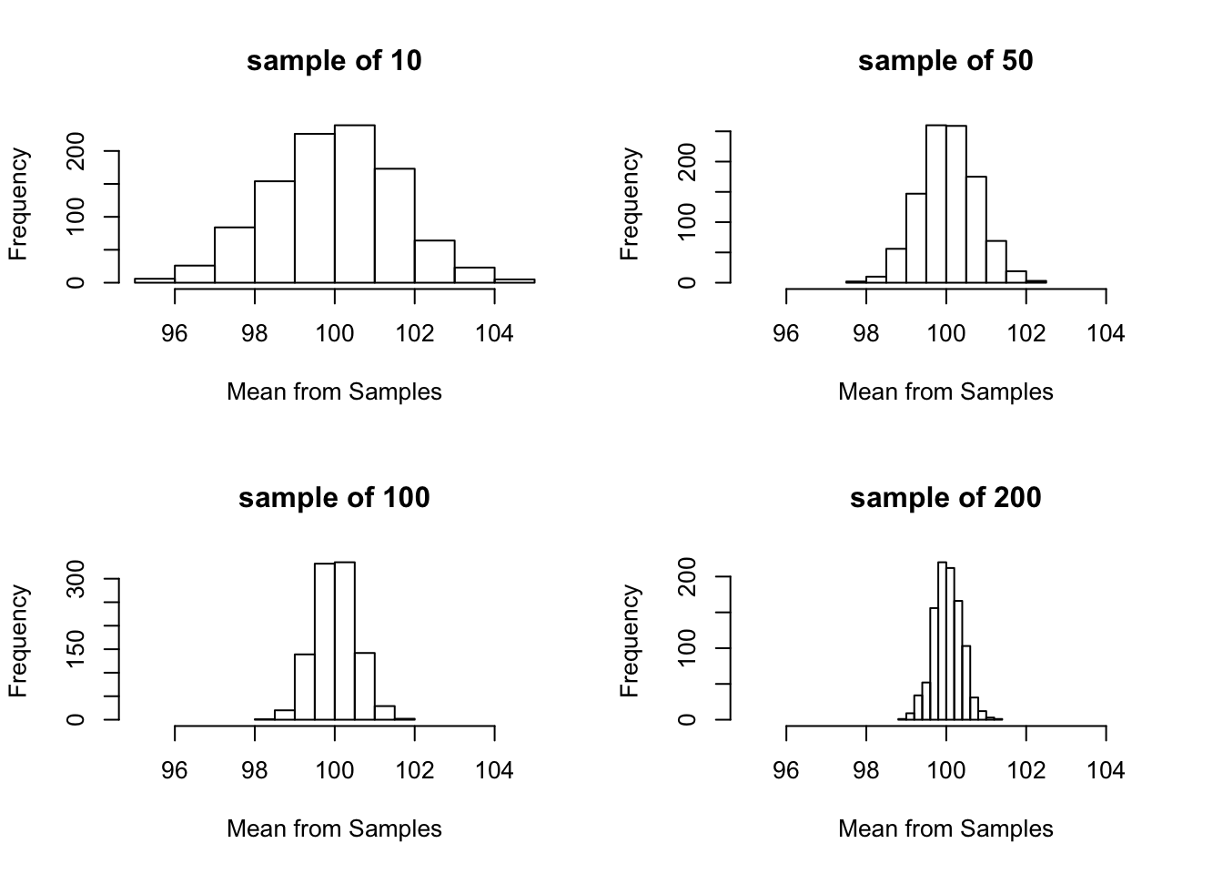
As our samples become larger the data becomes more and more tightly bunched around the true mean of the population. We can get accurate results from sampling a small share of the population, but all else being equal a larger sample is always nice.
So in order to understand the accuracy of sample estimate we calculate the sample error using this formula:
Standard Error = \(\frac{sd}{\sqrt{n}}\)
To put that in English, we are dividing how noisy the data we collected is by the sample size. When we talk about data in general and a normal distribution we talk about standard deviations. When we’re using a sample we want to use standard errors to measure the noise around the mean. That formula identifies two ways of getting more accurate results. Either we can get less noisy data, or increase the sample size. Generally, one can’t change how noisy the data is, so that indicates we want to collect larger samples if we know our data is more dispersed, and can use smaller samples if our data is less noisy.
Oh, and why do we talk the square root of the sample size? I don’t really know. I could probably look it up, and I’m sure I have in the past. But if I haven’t remembered it at this point I doubt it’s very important.
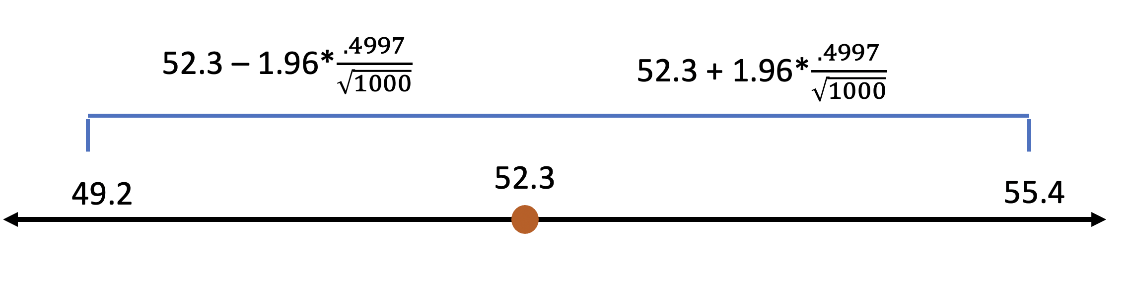
So what’s the standard error for the data we collected from our poll? The standard deviation is 49.97, and the sample size is 1000.
\(\frac{49.97}{\sqrt{1000}}\) = .04997
This is where I get annoyed in math textbooks, because I always want to scream “so what? What does that mean!?”
So I get it. That number doesn’t mean much on it’s own. But it allows us to calculate something really important. The standard error is critical to calculating a confidence interval, which gives us bounds on what we think the populations vote total is based just off the sample we collected.
12.1.3 Confidence Intervals
You know from the previous example that if the sample you took is representative (and lets say it is) that the value for that sample should be similar to the population. But you also know that if you took a different sample your result would probably differ slightly, maybe moving up and maybe moving down.
What you want to know then is how much error you expect around your estimate. How much would you expect a different sample to move up, and how much would you expect it to move down?
The central limit theorem helps us to predict that. Whatever value we get for our sample (52.3% voting for Duke) we can expect that result to be within 1 standard error of the population mean 68% of the time. We can expect it to be within 2 standard error of the population mean 95% of the time. And we can expect it to be within 3 standard errors 99.7% of the time.
That is to say it is possible the population mean wildly differs from the sample mean, but we generally expect them to be similar, and depending on how close the race is we can start to figure out the chances of Duke or Rover winning.
What do we need to calculate the confidence interval? Let’s take a look at the formula, which might look a little scary but actually isn’t that bad. Most of what we need to gather are actually ingredients we already have lying around the kitchen.
Confidence Interval = Sample Mean + \(Z * \frac{sd}{\sqrt{n}}\)
So that’s our standard error, which we calculated above, multiplied by something new called Z.
Remember from the central limit theorem and normal distributions that a sample we draw has a 95% chance of being within 2 standard errors of the population mean. We can also reverse that. A sample mean thus has a 95% chance of being within 2 standard errors of the population mean. But what a confidence interval does is it takes the sample mean and figures out how far around it 2 standard errors is because that lets us be 95 confident that the range contains the population mean.
Z essentially is the symbol for how many standard errors away from the mean that we want to calculate the values for. Why would we want to calculate any distance? Because we want to create a range within which we will be _% confident that the population mean falls. For instance, within 2 standard errors (or 1.96 standard errors technically) we can be 95% confident the population mean falls.
What that means for our example election is that we can be 95% confident that the true percentage of voters that will vote for Duke is somewhere between 2 standard errors above the sample mean, and 2 standard errors below the sample mean. Calculating those lets us say that the vote should fall somewhere between 49.2 and 55.4.
What does 95% confidence mean? It means we’re pretty confident. 95 times out of 100 we would expect the true population vote total to fall in that range, but we also have to acknowledge that 5 times out of 100 it wont. It could be higher, or it could be lower, but most of the time the final value will fall in that range.
Maybe we want to be more confident in our guess. We can be 99% confident that the population mean falls within 2.58 standard errors. That increases our confidence, but also widens our range of possible values.
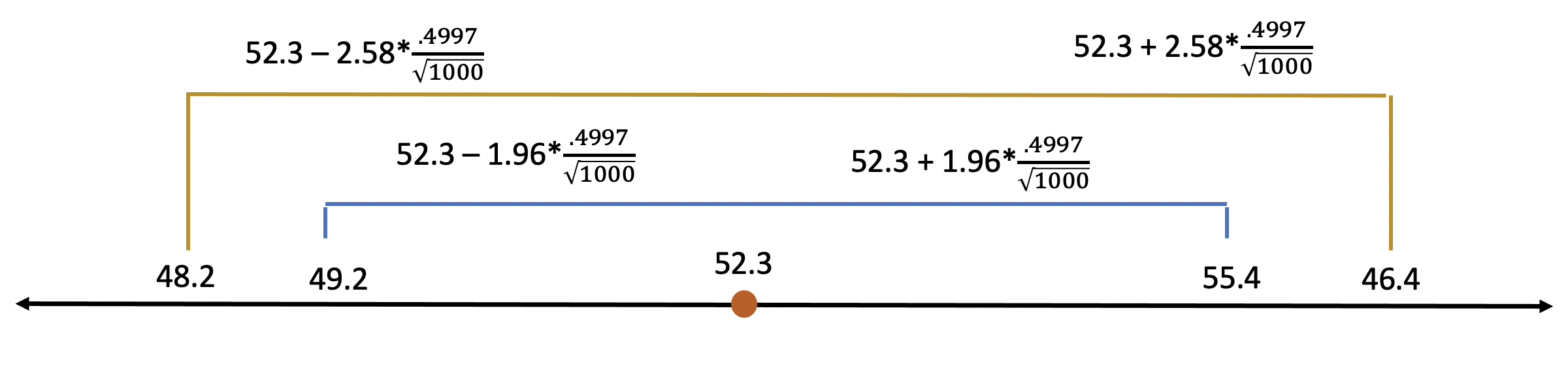
1.96? 2.58? Those numbers aren’t very intuitive and they just sort of have to be memorized through use. They refer to the specific number of standard errors a specific share of values fall within a normal distribution. I know I said above that 95% of values fall within 2 standard errors above, and that’s short of a short hand, but the actual value is 1.96.
| Percentage Confidence | Z Value |
|---|---|
| 80 | 1.28 |
| 90 | 1.645 |
| 95 | 1.96 |
| 98 | 2.33 |
| 99 | 2.58 |
Most typically we like to do things with 95% confidence, because that limits the chances of making an assertion that proves false, and when possible we like to be even more confident. But with polling data our sample sizes are typically too small to get meaningful estimates with more confidence.
But back to the important question. Can we declare Duke the winner or not? We know the percentage of our sample that voted for Duke, and we now have a confidence interval that gives us a range of values that the true percentage of voters might have voted for her.
To answer that question we need to calculate confidence intervals for both candidates.
Before our TV station declares a winner they want to be at least 95% confident that we have the winner right. So we’ll calculate a 95% confidence interval for Duke and Rover below.
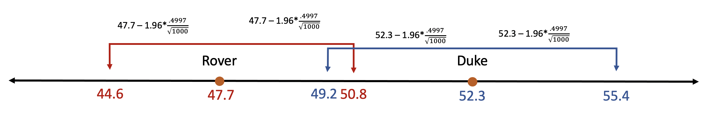
No, we can’t be 95% confident that Rover has won. She has more votes in our poll, but we think that her vote total in the population might be as low as 49.2 (the lower bound on her confidence interval). At the same time, we think Rovers vote total in the population might be as high as 50.8 (the upper bound on his vote total). If that’s true, Rover would win. Because the two confidence intervals overlap, we can’t be confident enough to say that Duke is going to win yet. We can’t declare the election decided based just on the evidence from the exit poll we already have.
But good news! while you were crunching the numbers from the first exit poll, another one was conducted and this time 2500 representative people were asked who they voted for.
The race has tightened slightly. Duke’s lead has narrowed slightly, now getting 52.08% of the vote compared to 47.92% of voters who supported Rover. But, remember, earlier we said that a larger sample would narrow our confidence intervals. Also, the standard deviation for the samples hasn’t changed, for what that’s worth. Let’s see if the network can declare a winner now.
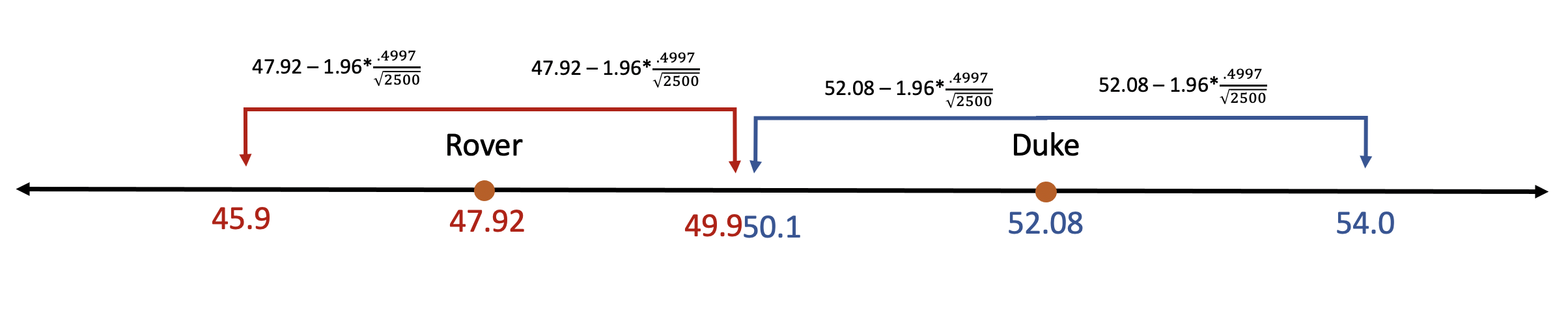
The network can now be 95% confident that Duke will win the election. We are 95% confident that Duke’s share of the vote in the population falls somewhere between 53.03% and 50.12%, and that Rovers proportion of the vote is between 49.88% and 45.96%. Even if Duke’s final vote is at the lowest end of that spectrum (50.12%) and Rover’s is at the high end (49.88%), Duke will squeak by with the win.
There is still a 5% chance that the vote total is above or below those intervals. Rover might get more votes than the upper bound of his confidence interval, but that would be considered a rare outcome so the network can feel confident (95% confident) in declaring the election decided. And they can actually feel more than 95% confident. If the final vote is outside the confidence intervals it is also possible that Duke will outperform her upper bound of 54.03, which would mean that the declared winner simply did better than we expected. That might not look great mathematically, but at least the network wont be embarrassed for calling the election too early. Thus, there’s only a 2.5% chance that the network would call the race for Duke, but Rover would end up winning.
12.1.4 Margin of Error
Often when you hear the results of a poll reported they wont mention the confidence interval. What you’ll often see referenced is the margin of error. Often it’s in the fine print. Let’s take a look at this random graphic I pulled from the internet for a poll in April 2020 about how Florida would vote in the presidential election.
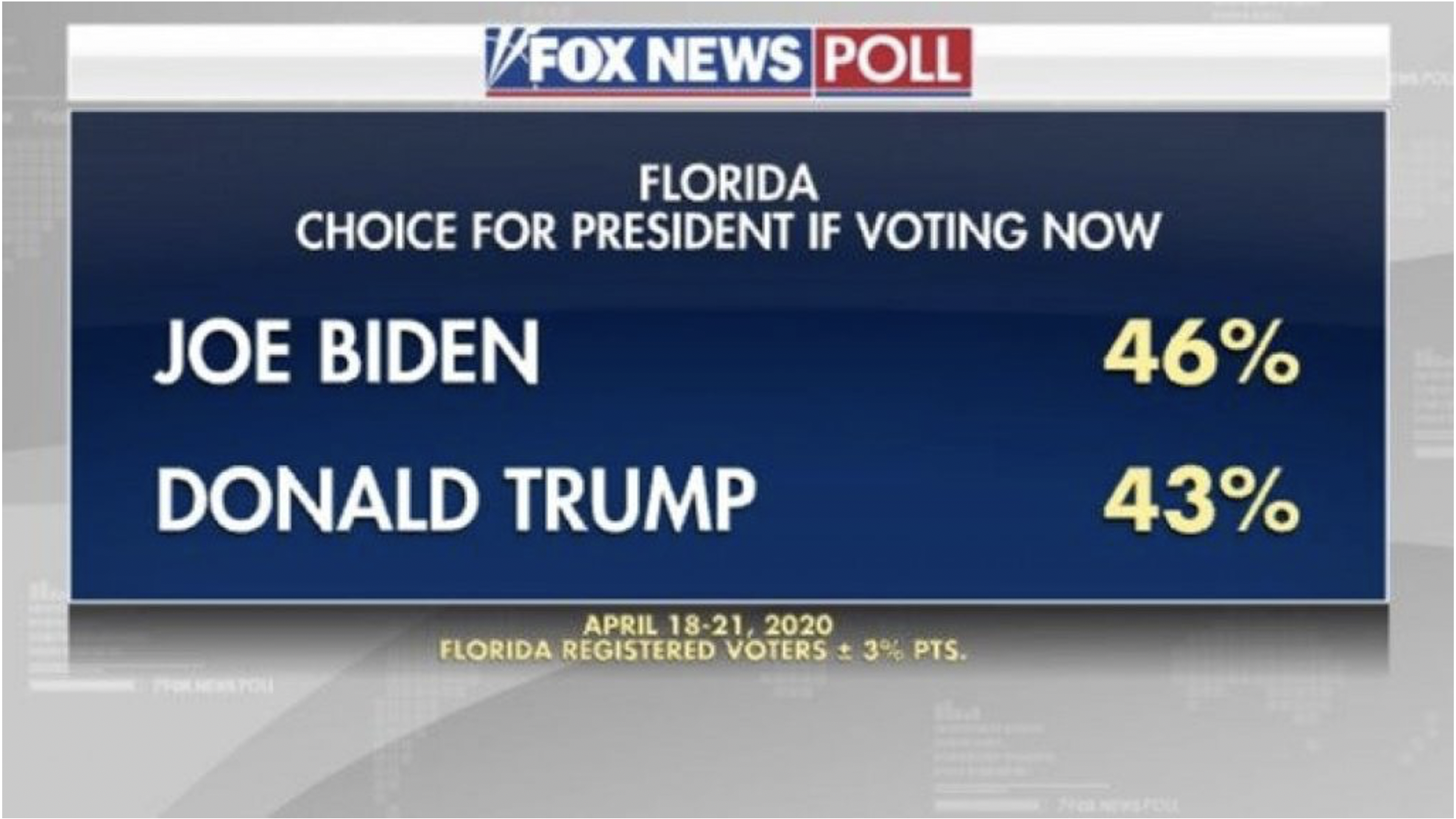
The big print goes to the headline takeaway: Biden leading in important swing state. But underneath that, in much smaller font, are some important details. The poll was conducted April 18-21. It was conduced for Florida Registered Voters (more on that later). And then there is the %+-% 3% points. That means the sample found 46% of registered voters in Florida planned to vote for Joe Biden, and 43% planned to vote for Donald Trump, with a margin of error of plus or minus 3 percentage points in the population.
What does that mean for our interpretation of the poll result? It means that the poll found that in the population the share of voters that would support Biden would be 46% plus or minus 3%, so between 43% and 49%, and for Trump the range would be 40% to 46%.
The formula for margin of error is essentially the same as what we used to calculate a confidence interval. When calculating a confidence interval we add it to the mean from the sample to provide a range. But for margin of error we just calculate the distance for those boundaries.
Lots of terminology I know, so let’s review.
Standard error measures the preciseness of a sample.
Standard Error = \(\frac{sd}{\sqrt{n}}\)
A confidence interval is the range of values that is expected to contain the population mean. We calculate it by adding the sample mean to the standard error times a measure for how precise we want the estimates to be.
Confidence Interval = Sample Mean + \(Z * \frac{sd}{\sqrt{n}}\)
And the margin of error is just the figure for how wide half the confidence interval is.
Margin of Error = \(Z * \frac{sd}{\sqrt{n}}\)
Why do we need a confidence interval and margin of error when they are essentailly telling us the same thing in different ways? In part, its because they’re used differently. News stations and pollsters often report the margin of error, in part to ensure their results are more interesting. Think about the graphic above from the poll of voters in Florida. Fox News discussed these results in part because it appeared to show that Joe Biden was leading in Florida, and he was in the poll. But was he really? The confidence intervals around the polls overlapped significantly, but saying that the race is virtually tied isn’t as interesting. Thus, and this might partially just be my skepticism, but margins of error are reported because they’re easier to ignore.
So you should try and understand them both, because they’ll both be used.
12.1.5 Good polls
Doing good polls is really complicated, in part because of the challenge of getting 1000 respondents to match a population. If the sample you use is not representative, the results don’t tell you anything about the population.
That becomes all the more difficult at election time when pollsters have to figure out not just what the American population looks like, but what voters will look like. We know that not every American is equally likely to vote. For instance, older, whiter, and college educated individuals are more likely to vote, so a good pollster has to account for all of those demographics and more in figuring out who to include in their sample.
One not only has to get the sample to match the pool of likely voters they expect, but has to get responses from those people as well. Certain demographics are less likely to respond to polls or surveys as well. In the chapter on sampling we talked about using weights to adjust the value of certain responses, but now you’re trying to adjust those values to match the predicted numbers of who will vote. Which is to say, it’s complicated.
This is part of what made the 2016 presidential election so difficult to accurately predict.
The New York Times in September 2016 ran a great article on exactly this topic. They took the sample poll data that they collected and gave it to 5 different pollsters to weight for them to match to their projections of likely voters in that year. Again, the same exact underlying data was used. What happened?
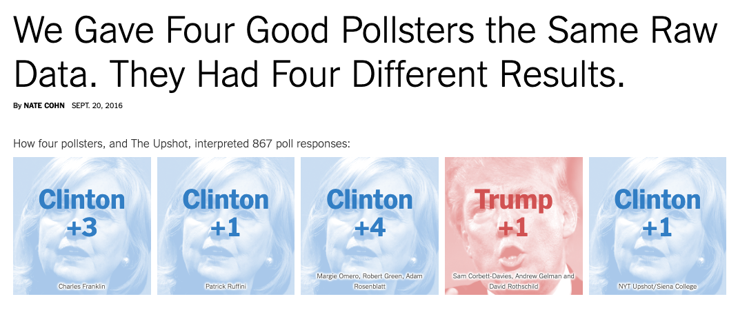
They got really different results! Why? Because the 5 pollsters all thought a different gorup of voters would show up to cast their ballots.
After Donald Trump outperformed his polls on election night it led some to declare that the pollsters didn’t know anything, and that would be unfair. Pollsters had a difficult time predicting the exact share of college educated vs those without a college degree that would vote in certain states in 2016, but most results were within the margin of error. What those challenges highlighted was the difficulty of predicting exactly who would vote in a given election, and the challenges of getting responses from a representative set of those voters.
One more word on the Florida polls we used in the graphic above. What was the sample there? Registered Florida voters. Not likely voters, however the pollster might define that, but registered voters.
Citizens are not an exact match for registered voters, because not all adults are equally likely to be registered to vote. And registered voters are not an exact match for likely voters, because not all registered voters are equally likely to vote. When you see a poll of registered voters that’s an important caveat to note. That’s easier for the pollsters to conduct because they don’t have to determine who is likely to actually cast a ballot on election day, but it also means their results will be less likely to exactly match what occurs in the election.
12.2 Practice
We’ll see confidence intervals and sample errors a lot in future sections, but in general R will calculate them for us as part of a different operation. But it’s worth practicing calculating them by hand in the meantime.
Let’s use a subset of the data from a Pew survey, and I’ve selected the least controversial question I can: “Are you looking forward to the presidential election this fall?”. Respondents either said Yes, they are looking forward to the election, or no, they aren’t. Let’s look at the data and come up with a confidence interval for our estimate of what share of the American public is looking forward to the election.
election <- read.csv("https://raw.githubusercontent.com/ejvanholm/DataProjects/master/Anticipation.csv")
head(election)
## QKEY Anticipate AnticipateYes AnticipateNo
## 1 100197 Yes 1 0
## 2 100260 Yes 1 0
## 3 100446 Yes 1 0
## 4 101437 Yes 1 0
## 5 101472 Yes 1 0
## 6 102932 Yes 1 0The variable QKEY is a unique id for the respondent, the variable Anticipate is a categorical variable for whether they responded Yes or No, and AnticipateYes and AnticipateNo each record as 1s and 0s how they responded.
So if we calculate the statistics by hand we need our formulas. Let’s concentrate on the column AnticipateYes first.
Standard Error = \(\frac{sd}{\sqrt{n}}\)
To calculate the standard error we need the sample size, which we can get with the command nrow() and the standard deviation using sd(). We’ll also need to take teh square root of the sample size, which we can do with sqrt().
## [1] 0.005313019Since we’re going to use the standard error in later calculations, it could make sense to save it here so that we don’t have to reenter that formula later.
Confidence Interval = Sample Mean + \(Z * \frac{sd}{\sqrt{n}}\)
Let’s calculate the margin of error, and we’ll use 1.96 as the value for Z. We can save that value as me.
Margin of Error = \(Z * \frac{sd}{\sqrt{n}}\)
## [1] 0.01041352The margin of error is .01. So let’s turn that into a 95% confidence interval by adding and subtracting it from the sample mean.
## [1] 0.7693654## [1] 0.7797789## [1] 0.7589518So our 95% confidence interval would stretch from 75.9% to 78%. 77% of the sample said they were looking forward to the election, and we are 95% confident that between 76% and 78% of the population feels that way.
That was doing the math all by hand. We can also have R do all those steps for us, but we’d have to use something called a package.
Packages are sort of like apps on an iPhone. R is capable of doing all kinds of actions and procedures, but some aren’t avaliable in what is called base R. Base R refers to the set of packages and operations we can do with R straight out of the box. Packages are additional commands we can use if we download them. Just like everything in R they’re free, but we still have to acquire them.
It’s similar to apps on an iPhone. Your iPhone doesn’t come loaded with every app, because taht would be more than anyone needs and would take up all the memory. Rather, it comes preinstalled with some of the more common things people need, and you can customize from there. So this is going to be a vinette on packages in R, that’ll end with calculating confidence intervals easier.
So there’s a manual way of checking whether a package is installed on your computer. On the bottom right portion of your screen, where a graph usually pops up, there is another tab for packages.
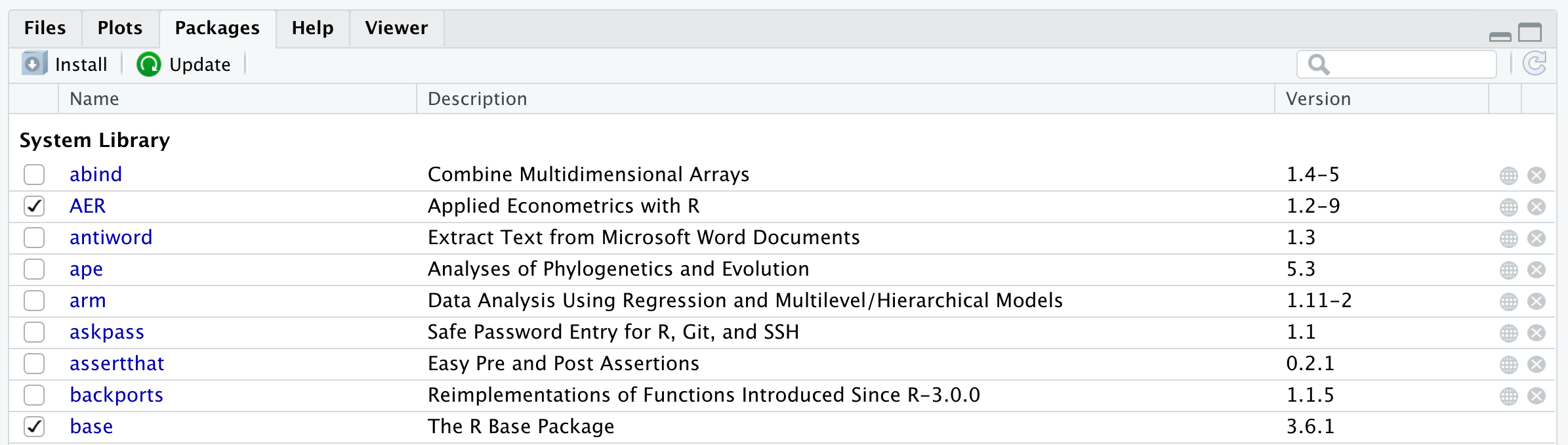
If you click on yours it probably wont match exactly what you see in the picture above, because I’ve dowloaded a few packages in my days. But there should be a few names in the picture that are on your computer already.
There is a search icon in the cornoer of that box where you can search for a package name to see if it is installed. The package we’re going to install is called rmisc, which you can search for but it shouldn’t already be installed. Let’s fix that though.
To install it we’ll use the command install.packages() with the name of the package we want in quotation marks.
Once you run that line of code rmisc should show up on your list of packages now. That’s how you download an app from the app store, just run the line install.packages with the name of what you want. Once it is installed it is installed for life (unless you uninstall it), so oyu only need to do that once.
How would you find a package you want? Generally it will just come up when you search for how to do something in R, and someone on the internet will suggest using some package. You typically don’t go hunting for packages as a way to discover new things to do, they’re generally a solution to a problem you already have.
Okay, once the package is installed we need to load it. The command for load is library(), where you put the name of the package inside the parentheses.
Okay, now we can use the commands that come with Rmisc, such as a command that can produce a confidence interval for us in one step. That command is called CI(), and we just need to give it the name of the data set and column we want a confidence interval for.
##     upper      mean     lower
## 0.7797807 0.7693654 0.7589500
That matches what we calculated above manually, but is a lot easier.
I’d recommend redoing those steps for the column AnticipateNo just for practice, if you’re interested.