10 Descriptive Statistics
This introduction doesn’t actually introduce the topic, but is rather meant as a reminder about how this and subsequent chapters will be structured. The first half will describe the concepts used in the chapter, and why they’re useful. There wont be any coding shown in that portion of the chapter, but there will be examples of the type of output we’re discussing. The text is meant to be read just like any other book.
The second half of the chapter, the practice section, will walk students through creating all of the statistics we describe in the first half using R. The second half of the chapter should be read “actively” while practicing the code yourself. Most of learning to code is just taking code someone else has produced and practicing it until you know it.
10.1 Concepts
Descriptive statistics are a first step in taking raw data and making something more meaningful. The most common descriptive statistics either identify the middle of the data (mean, median) or how spread out the data is around the middle (percentiles, standard deviation). The statistics we calculate as descriptive statistics will be useful for many of the more advanced lessons we’ll encounter later, but they are important on their own as well.
Descriptive statistics are useful for exactly what it sounds like it would be: describing something. Specifically, describing data. Why does data need to be described? Because raw data is difficult to digest and a single data point doesn’t tell us very much.
10.1.1 Data
We’ve used the word data in a few different ways throughout this book. Data can be words, data can be numbers, data can be pictures, data can be anything. But one of the most common associations of the term is with a spread sheet. If I tell a colleague to “send me the data” I probably mean send me a spreadsheet with the information we’re discussing. When we discuss using data in the upcoming chapters, we’re discussing using a spreadsheet. Just so that we can full understand that use of the term, let’s discuss the anatomy of data/spreadsheets in a little more detail.
Let’s start by looking outside of R at the most popular spreadsheet program available: Excel.
Data is made up of rows and columns. Rows run from side to side on the sheet, while columns go up and data. Each data point falls into a cell, which can be identified by the exact row and column it has in the data.
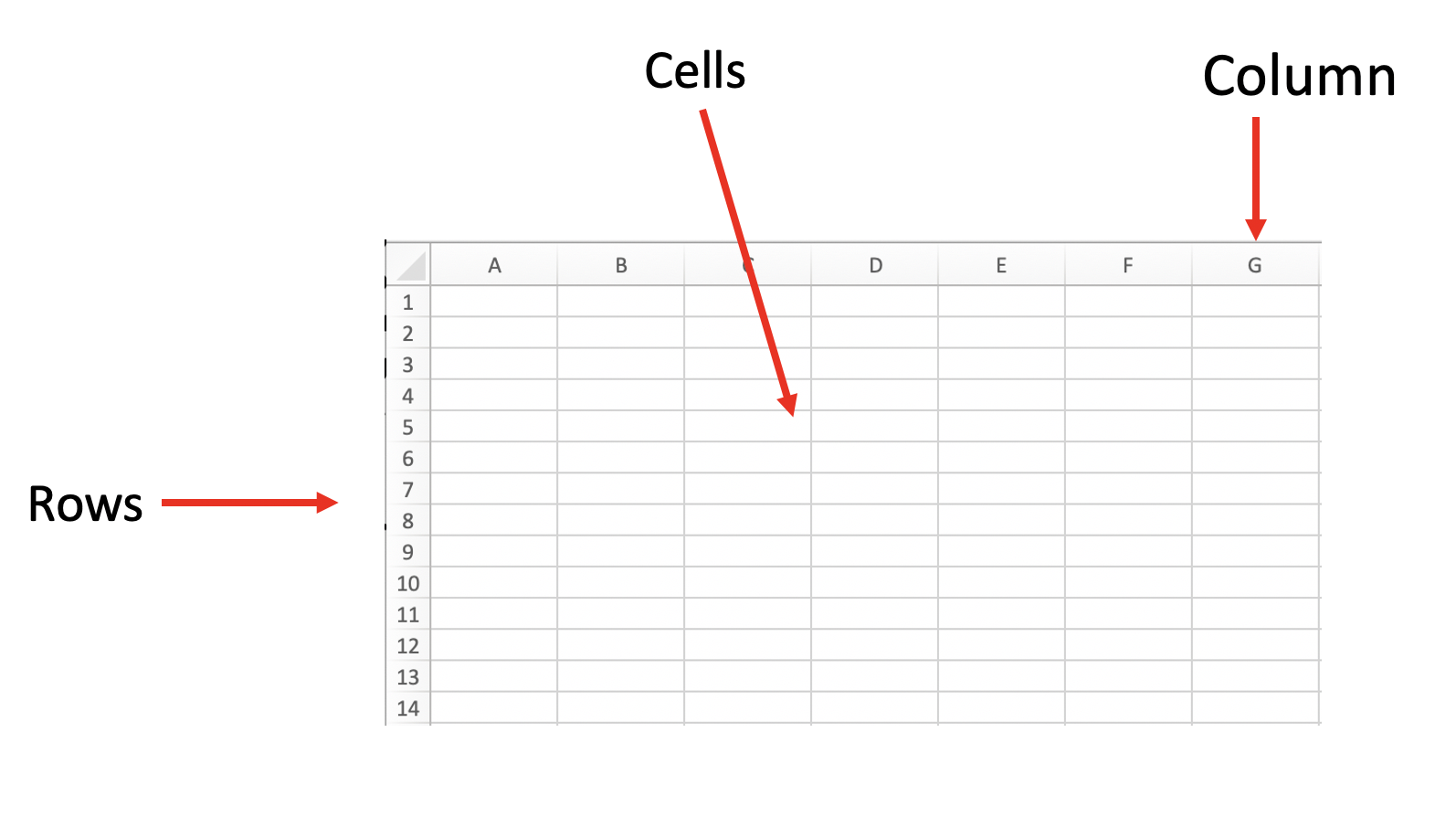
We want to label our columns with a short phrase that indicates what the data points in that column represent (Age, Education). Each column holds the same information for all of the rows in the data, while each row has the data for a single observation. Below I show a few rows for some made up data. The first person in the data is 18, has 12 years of education, and is not married. The 7 people in the data are 18,45,32,74,52, and 34 years old. Each column has a name, and typically rows just have a number.

There are a lot of names for a spreadsheet. You can call it a data set, or a data frame, or just the data. Data set and data frame are pretty common, and I’ll slip back in forth on what I call it.
10.1.2 Summary Statistics
Okay, so why does data need describing then? There are a few good reasons to use descriptive statistics. One is in order to condense data and another is for comparisons. We’ll talk about both in this chapter, and we’ll keep coming back to those words: condense and compare.
Let’s say my child is a student at Wright Elementary in Sonoma, California. Every year schools take the same standardized math test, and when the scores come out I want to know whether my school is good or not. Finally the reporting day arrives and the results are announced: Wright Elementary scored 668.3.
Is that good or bad?
I don’t know. That’s just an absolute figure, which doesn’t tell me anything about how any other school did.
So I want to know how my school did, not just in the absolute sense of how many points it earned, but relative to all other schools in the state.
I call the head of the Department of Education and I say “show me the data!” and they do…
##   [1] 690.0 661.9 650.9 643.5 639.9 605.4 609.0 612.5 616.1 613.4 618.7
##  [12] 616.0 619.8 622.6 621.0 619.9 624.4 621.7 620.5 619.3 625.4 622.9
##  [23] 620.6 623.4 625.7 621.2 626.0 630.4 627.1 620.4 628.7 626.9 629.8
##  [34] 625.6 626.8 628.2 630.2 625.3 630.1 627.1 628.7 635.2 627.7 636.2
##  [45] 631.0 629.4 631.2 628.9 629.5 632.6 633.7 627.1 630.7 634.2 629.7
##  [56] 630.5 633.0 627.0 627.6 632.5 636.7 635.8 636.7 632.9 633.1 629.6
##  [67] 636.2 630.5 636.7 631.5 636.6 631.1 633.6 636.2 638.7 632.1 633.5
##  [78] 626.1 630.0 636.6 638.2 634.8 638.7 638.3 638.3 627.8 641.1 641.4
##  [89] 637.7 637.9 636.2 633.8 630.4 629.8 642.7 639.3 636.0 640.4 646.2
## [100] 638.1 639.6 640.5 638.2 635.9 638.8 637.6 637.8 638.1 638.3 645.5
## [111] 636.7 639.9 643.3 643.0 636.9 641.8 643.6 644.3 642.3 644.7 642.6
## [122] 647.4 644.6 632.9 644.1 643.8 647.1 647.9 645.1 642.8 634.3 653.8
## [133] 641.7 636.1 643.9 636.7 639.4 645.7 644.7 643.1 644.1 640.2 647.3
## [144] 633.7 633.1 643.4 646.4 647.2 646.0 639.5 641.5 649.7 651.2 645.2
## [155] 644.0 649.4 648.2 646.1 651.6 649.5 643.8 645.8 643.6 651.0 648.4
## [166] 647.7 645.1 654.0 652.8 652.3 643.4 649.2 648.1 647.1 645.8 646.5
## [177] 645.8 647.7 650.0 645.7 649.0 650.7 648.3 640.8 655.9 649.4 651.8
## [188] 647.5 655.8 647.8 652.6 649.5 653.7 647.5 644.5 649.6 651.9 648.9
## [199] 650.1 653.1 654.6 651.5 653.7 653.3 652.1 651.8 651.3 656.8 650.6
## [210] 648.6 653.5 656.5 655.5 656.2 647.6 660.1 652.7 649.7 649.6 655.2
## [221] 657.7 653.1 657.6 649.1 659.8 649.6 655.8 658.7 655.2 654.4 657.9
## [232] 651.9 650.2 656.9 656.4 656.7 653.3 649.9 642.2 650.9 655.6 655.3
## [243] 660.5 657.3 659.0 652.7 662.5 656.3 663.2 656.2 660.4 656.0 658.8
## [254] 658.8 659.4 658.4 647.1 660.6 652.8 654.6 659.8 661.6 660.9 664.1
## [265] 650.8 663.6 658.3 661.0 659.5 661.3 663.5 661.7 673.4 659.5 661.5
## [276] 663.4 655.7 667.0 663.0 658.4 657.5 659.3 662.6 666.8 661.3 668.3
## [287] 670.1 661.8 659.3 657.0 661.6 654.6 665.4 665.8 663.9 665.8 662.3
## [298] 664.0 663.4 674.2 660.9 667.4 661.5 667.4 664.0 663.4 665.3 660.4
## [309] 661.3 664.1 661.9 669.5 661.2 665.8 671.3 666.8 662.4 666.6 664.6
## [320] 662.7 667.9 666.0 666.6 675.7 671.0 664.5 668.5 669.1 671.6 672.4
## [331] 672.1 669.7 657.7 665.4 674.1 669.5 666.5 670.7 670.8 668.6 671.3
## [342] 668.0 668.3 671.8 665.7 663.6 674.6 670.7 664.2 671.6 668.0 670.2
## [353] 676.5 670.1 672.2 675.7 669.3 667.0 671.5 670.5 666.6 676.6 677.3
## [364] 672.5 669.8 668.4 672.2 679.3 679.9 673.2 681.1 675.5 677.4 673.2
## [375] 671.5 678.6 674.7 682.2 676.2 680.8 679.4 674.4 676.7 679.8 681.8
## [386] 674.7 674.0 682.5 684.9 679.5 678.0 684.3 682.3 688.2 680.2 687.4
## [397] 683.7 679.9 690.3 681.3 686.6 688.6 695.0 690.1 692.0 694.9 691.7
## [408] 695.3 689.3 695.7 697.3 701.1 703.6 699.9 701.7 707.7 709.5 641.7
## [419] 676.5 651.0
That’s a lot of data! Number after number is in there, and somewhere in the list is the score from Wright Elementary at 668.3. Okay, so I’ve got the data, now what do I do to understand the data. Just having raw data wont help me make better decisions unless I can organize it in some way to answer my question.
Take a look at that list again then, does 668.3 look high or low? It’s lower than the first number, but higher than the second and third. But I don’t want to take the time to compare my school to every other school individually. That would be exhausting just with the 420 schools that are in the state of California. Rather than doing 420 individual comparisons, let’s have R do some math for us.

If I want to understand how well Wright Elementary is doing, it’d be useful to summarize the data in some sort of clear way. I can start by measuring the middle of the data, using the average or the mean.
10.1.2.1 Mean and Median
Mean is just a mathy word for average that you’ll rarely see outside of math classes. We can use the two terms interchangeably in this book, but in most math it’ll just be referred to as the mean.
To calculate the mean, you add up all the individual values and divide it by the total number of observations. Of course, you’ll never have to do that again because R can do it for you a lot quicker than you can. But it’s still worth understanding what the gears in the machine are doing: adding up all the values in a column, and dividing it by how many rows there are.
Average is perhaps the most commonly discussed statistic in the world. Every year you’ll hear reports about whether test scores are increasing or decreasing based on statewide averages. Sports fans know the average number of points their favorite basketball player scores or the batting average of baseball players.
Average can to some degree be taken as the expected value from the data. If you took a random data point, your best guess might be that it would be close to the average. If you go to a basketball game and the best player averages 30 points, you probably intuitively expect them to score about 30 points. It should be stressed that they probably wont. Picking a random data point or watching a random game doesn’t mean the figure will be anywhere near the mean. But it sets your expectations and provides you some guidance for the future.
Do you expect the food at a restaurant that averages 4.5 stars on yelp to be better than one that has 2.5 stars on average? The mean indicates something about the overall values in a data set, even if it doesn’t guarantee that any individual experience will be different.
So what the mean does is condense all of our data into one figure that tells us something about the middle of that data. And in this case the mean of our data is 653.3426.
And my kids school got 668.3. Great, that means my kids school is above average!
Does that mean Wright Elementary is better than half of the schools in the state? Not exactly. Sometimes the mean value of data will be the exact middle of all the values, but sometimes it wont. On the other hand, another measure for the middle of the data will be: the median.
The median is the exact middle of our data. If we have 3 numbers in our data, it’s the 2nd highest one. If we have 9 numbers, it’s the 5th highest. No matter what the highest and lowest numbers are in our data, the median will always be the middle number. If you have an even number of numbers it’s the average of the middle two.
Let’s use an example to describe why we might want to look at both the mean and the median.
If the average test scores in a given school district are increasing from one year to the next, does that mean every school is improving? No. Let’s take 5 hypothetical schools for some school district, and change their scores a few different ways to see how the average shifts.
| School | Test Score |
|---|---|
| A | 320 |
| B | 400 |
| C | 510 |
| D | 640 |
| E | 750 |
| Mean | 524 |
So to start the average test score for the 5 schools is 524. Let’s increase the average test score by 10 points in 3 different ways.
| School | Original | Change 1 | Change 2 | Change 3 |
|---|---|---|---|---|
| A | 320 | 330 | 320 | 300 |
| B | 400 | 410 | 400 | 400 |
| C | 510 | 520 | 510 | 500 |
| D | 640 | 650 | 640 | 600 |
| E | 750 | 760 | 800 | 870 |
| Mean | 524 | 534 | 534 | 534 |
In the column labeled Change 1 all of the schools increase their scores by 10 points, so the average test score increases by 10 points in turn. Everyone is doing better.
In the second column only school E has improved its score though, from 750 to 800. However, to calculate the mean we just add together all the values and divide it by the number of rows, so regardless the average score still rises. The third change is even more stark - Schools A, B, C and D all had decreases in their scores, but because School E did so much better the average test scores for all the schools increased!
Now imagine being an administrator for this school district, and hearing that average test scores have risen for the district. That should be good news. But as we just showed, that can mean a lot of different things about the data. Depending on which scenario occurs most of your schools are either improving or declining, despite the outcome being exactly the same. The average is a useful starting point to understanding our data, but it’s never sufficient on its own.
We have 5 schools, so the median figure will always be the 3rd highest test score.
| School | Original | Change 1 | Change 2 | Change 3 |
|---|---|---|---|---|
| A | 320 | 330 | 320 | 300 |
| B | 400 | 410 | 400 | 400 |
| C | 510 | 520 | 510 | 500 |
| D | 640 | 650 | 640 | 600 |
| E | 750 | 760 | 800 | 870 |
| Mean | 524 | 534 | 534 | 534 |
| Median | 510 | 520 | 510 | 500 |
In one of the scenarios the median stays the same (Change 2), in one it decreases (Change 3), and in one it increases (Change 1). That’s in contrast to the mean, which increased in all 3 scenarios. Here the median seems like a better measure of how the school district is changing, depending on which set of changes have occurred. However, the district might want to just report the mean because scores increasing looks good for all the officials! However, if they ignore the underlying change they may not understand what is occurring at the schools.
Which isn’t to say that the mean should never be used. It tells us something about the data too, and it’ll often be used in the calculation of other mathy stuff later in the book. But understanding the difference can help you to sniff out times when someone might be using statistics to lie or trick you.
There’s a famous hypothetical of Bill Gates walking into a soup kitchen where there are 9 homeless people that have zero wealth. Bill Gates of course has nearly infinite wealth ($113 billion as of my Googling), which means the average wealth of people in the kitchen is now 113 billion divided by 10. So each homeless person is now worth $11.3 billion? No, they still have zero dollars, but the average has changed. The median on the other hand is still 0, as the 5th most wealthy person in the room still has 0 dollars.
The mean and median are often misunderstood conversationally .
There’s a famous joke attributed to the comedian George Carlin that is shown below:
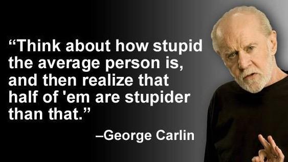
Are half of people stupider than the average person? Not necessarily, but 50 percent of people are stupider than the median smartest person. That makes the joke a bit more complicated though for the average person to understand.
10.1.2.2 Distribution
The median in the testing data is 652.45. That’s not far from the mean, 653.3426, but it’s not exactly the same either.
Whether the mean is equal to, above, or below the mean is a good indication of whether your data is skewed. If the mean and median are equal it’s a sign that the data is evenly distributed, and both figures are equally good at describing the middle of the data.
Skew just means not symmetrical, which in this context means that the distribution doesn’t fall evenly around the mean and median. The most famous distribution is the normal distribution, where the data is evenly distributed above the mean and the median. A fairly normal distortion is displayed below, with a mean and median of 100.
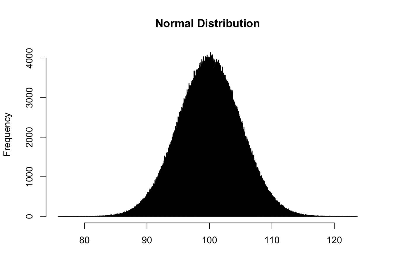
Normal distributions are really important for some of the mathematical stuff we do later. For now we can just accept that it’s important because it’s what we compare all distributions to, to understand how close or far from a normal distribution they are. Why we compare it is sort of hard to understand unless you know the magical powers that a normal distribution has, but that’s for a later chapter.
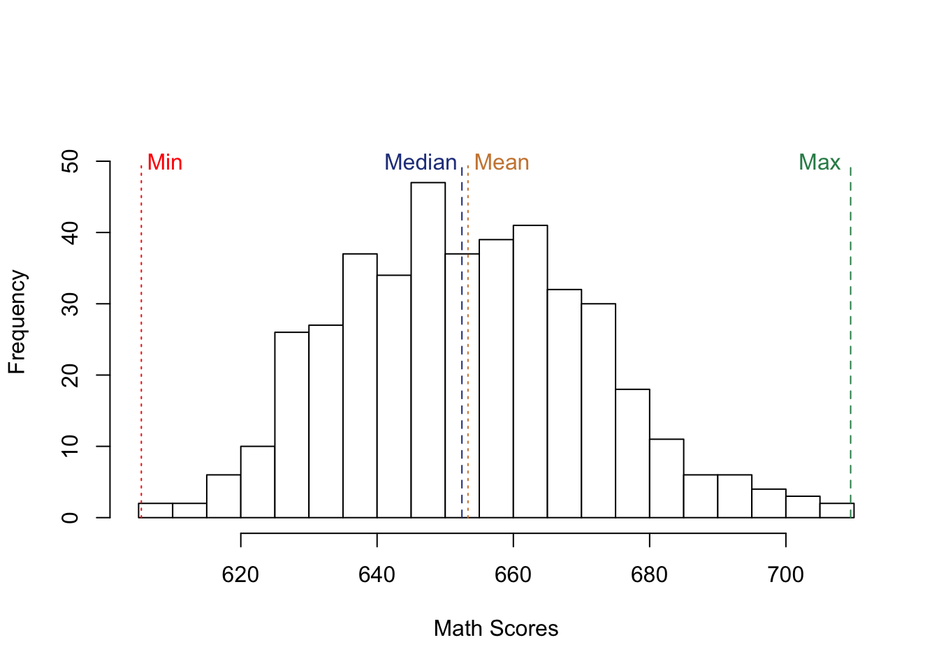
So let’s take a look at the distribution of all of the values from math scores in California. And we can add labels to show where the mean and median sit as well.
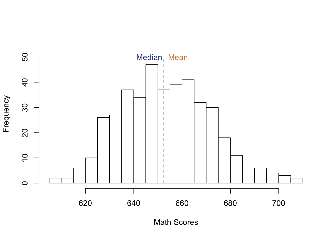
The first thing that might jump out at you is that this doesn’t look exactly like the normal distortion I showed above. It’s more lumpy in places, and it’s not quite evenly distributed above and below the median and mean. But the mean and median are still fairly close together. They can get much further apart with heavily skewed data.
Data can be skewed to the right, as shown below (we say skewed to the right because the “tail” of the data is pulled out to the right side).
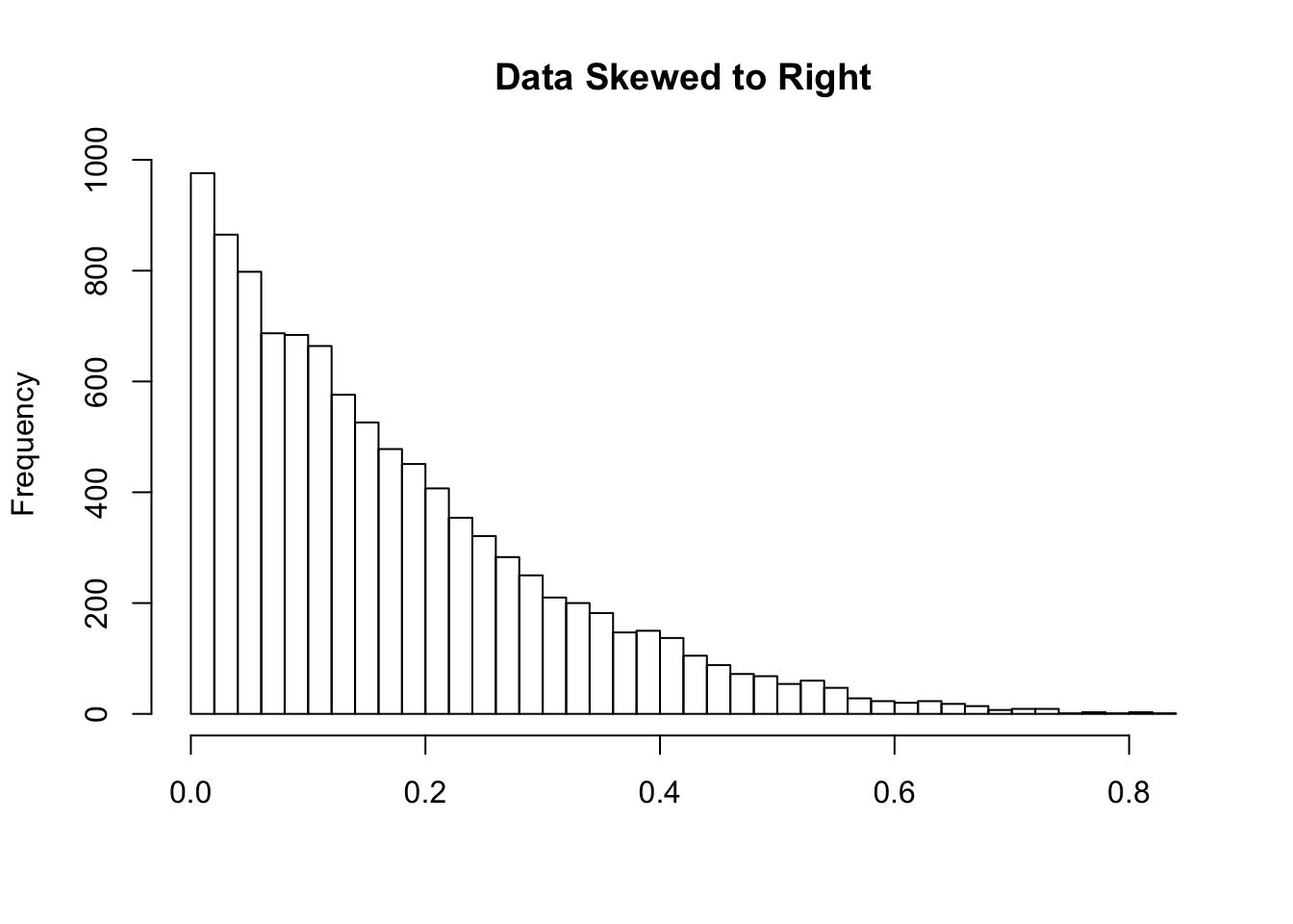
What happens to the mean and median in that case? Let’s plot it again and see.
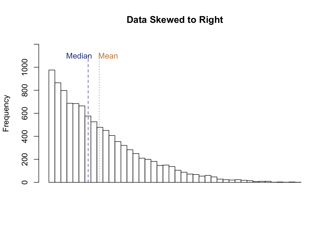
The mean is to the right of the median, another indicator that the data is skewed to the right.
Data can also be left skewed.
set.seed(3)
x <- rbeta(10000,35,2)*10000
hist(x, main="Data Skewed to Left", xlab="", breaks=50, xaxt = "n", ylim=c(0, 800))
segments(mean(x), 0, mean(x), 700, col="peru", lty=3)
segments(median(x), 0, median(x), 700, col="royalblue4", lty=2)
text(median(x)+130, 700, col="royalblue4", labels="Median")
text(mean(x)-130, 700, col="peru", labels="Mean")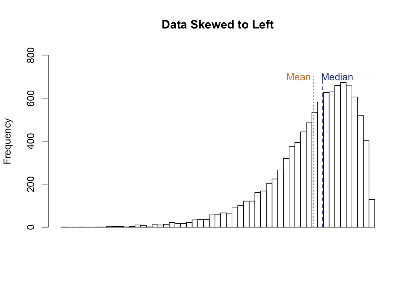
Here we see the data has a looooong tail to the left, and the mean is to the left of the median.
Skewed data comes up pretty often in the real world. For instance, let’s look at the distribution of income in the United States.
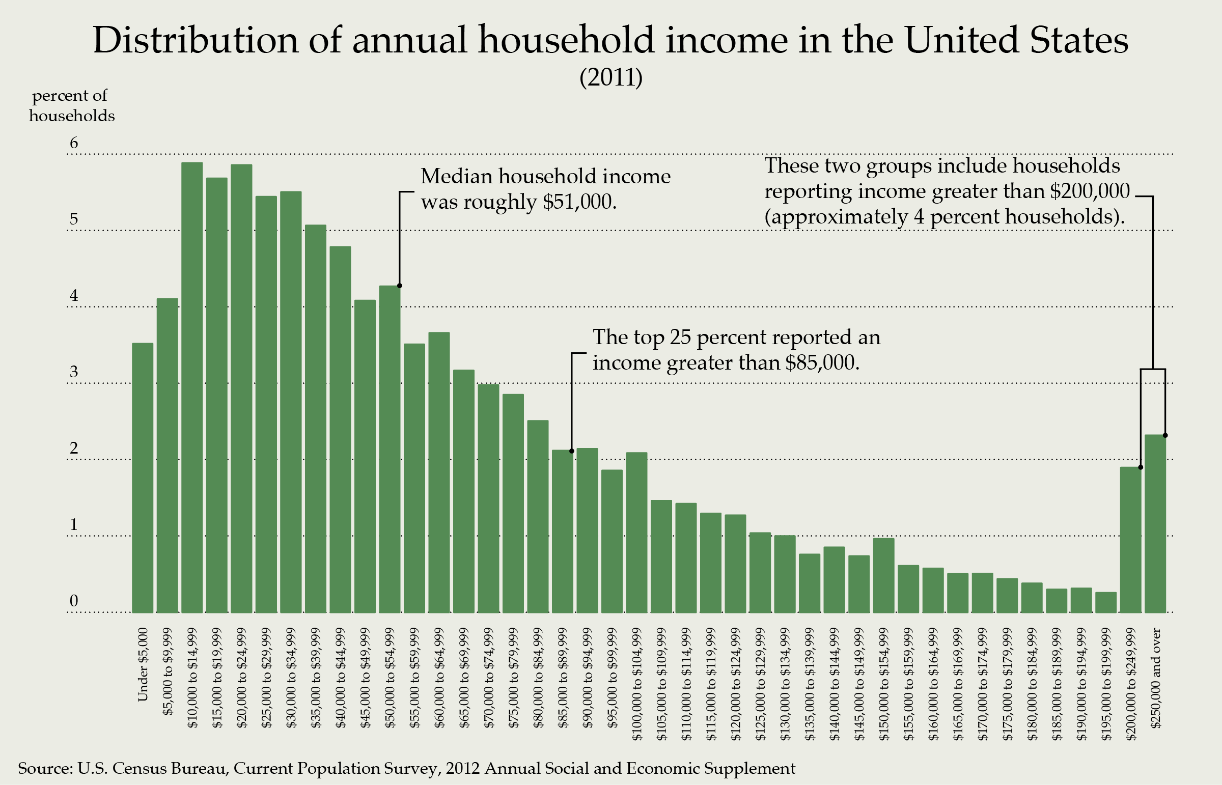
Income is heavily skewed to the right, which means the mean is above the median. We more often talk about the median income of citizens than the mean because the mean can increase primarily as a result off the wealthy becoming wealthier. If we concerned about how the average American is doing, median is actually a better measure to understand their status.
So a basic rule of thumb is to look at the mean and the median. If they’re the same you can just use the mean, that’s more easy for the average reader to understand. If they differ significantly report them both, or just report the median.
10.1.2.3 Mode
We’ve talked about two measures of the middle so far: the mean and median. There’s one more measure that is a little less common, the mode, which can be overlooked in part because it’s used less in quantitative studies.
Mode is the most common value in a list of data. It wouldn’t be a great way of analyzing the data on test scores in California. There the mode is 636.7, which appears twice, but that doesn’t help us to understand what schools are good or bad, it just tells us the most common score. Where it is more useful is with characteristics in our data, particularly if we’re trying to assess what the most common feature is. I wouldn’t want to talk about what the average color of hair is for my students, but rather what the most common hair color is. Or in a more applied setting, I might want to report what the most common race of respondents to my survey is, rather than their average race.
Let’s go through some examples where mode was (or would have been useful).
In 1950 the US Airforce was designing a new set of planes; in order to ensure that they would be comfortable for their pilots bodies, they took measurements of 4,000 pilots across 140 dimensions. That produces a lot of data! And with those measurements they fit the cockpit to the average pilot in the force: the average leg length, arm length, shoulder width, etc.
What happened? It was a disaster. The plane fit the “average” pilot, but no pilot actually fit the dimensions of the numerical average. It was uncomfortable for everyone, because it was designed for a composite individual that didn’t exist. A better strategy may have been to identify the modal pilot with the most common sets of features, and design the cockpit for that pilot. That might have not been comfortable for all the other pilots, but at least someone would get a plane they could control.
Similar question then - who is the average American? I often hear that politicians are attempting to appeal to the average American, but I don’t actually know who they are. If we take the numerical average of the nation’s demographics, they would be 51% female, 61.6% non-Hispanic white, and 37.9 years old. That doesn’t really sound like anyone I know though. What we mean by average American is actually most common American, which would indicate what we really want to find is the modal American. But that phrase sounds a bit clunky, so maybe it wont catch on.
If you’re interested in knowing who the modal American is there’s an episode of the podcast Planet Money that discusses that question and has a fairly interesting answer.
10.1.2.4 Outside the middle
So we have three measures for the middle of our data, each of which might be useful depending on the question we’re attempting to answer and the distribution of our data. But we’re not just concerned about the middle. The middle is a good place to start, but we’re also concerned about more than the middle. Mean and median are great for condensing lots of data into a single measure that gives us some handle on what the data looks like, but they also mean ignoring everything that is far away from those points.
Let’s return to figuring out whether Wright Elementary school did well on the math test or not. We know their score is above the average and the median by a few points. But that’s all we know so far.
Are they the best school in California? The highest value in our data is called the max or maximum, and so the max value is the school we would say did best. Was that Wright Elementary? Sadly (for their students), no. Los Altos got a 709.5, the highest score in that year.
At the other end of the spectrum would be the min or the minimum, which as you’re probably guessed is the lowest value in the data. In the case of the test score data that was Burrel Union Elementary with 605.4. The min and the max are useful points to give you a feel for how spread out the data is, and perhaps what a reasonable change in the data might be. It probably wouldn’t be a good idea for the principal of Wright Elementary to set a goal of adding 200 points to their math test score the next year, since that would far exceed what any school had achieved. A better goal might be a small improvement, or to match the best school in the state.
10.1.2.5 Relative Figures
So we can describe the middle (mean, median, mode) or the ends of our data (mix and max). Those are all really valuable for getting a quick look at your data, and they’re among the most common descriptive statistics used in research.
Another way of quickly summarizing your data would be to split them into percentiles. Earlier we referred to the score at Wright Elementary as a absolute figure. The score of 668.3 didn’t mean anything on its own, it was just the value we had. That’s in contrast to what are called relative figures, which tell us something implicitly comparative about the data
Percentiles don’t tell you what any one school in the data scored, but rather where a school is relative to all others in the state. In order to calculate percentiles, you essentially sort all of the values from lowest to highest, and put them into 100 equally sized groups. If you had 100 numbers in your data, the lowest number would be the 1st percentile, the second number would be the 2nd percentile, and so on. If you had 1000 numbers in your data, the lowest 1/100 (or the lowest 10) would be in the first percentile, with higher numbers sorting into higher percentiles.
The benefit of reporting percentiles is that they take absolute figures, which often don’t mean anything on their own, and turn them into something that tells you the relative rank of the figure compared to everything else. For instance, I see percentiles every time I take my toddler for a health check up, after they weigh and measure her. The fact that she was 27 inches tall doesn’t mean a lot to me, because what I really care about is whether she’ll be taller than her classmates at daycare. That’s why they also report her percentile height for kids of her age and gender - so that I know whether she’s taller or shorter than other similar kids.
We’ve already met one percentile earlier. The median represents the middle value in our data, so it is also the 50th percentile. If your kid is the median height that would mean they were taller than 50 percent of kids of a similar age, but also shorter than the other 50 percent. If they are 70th percentile, that would mean they are taller than 70 percent of other kids, and shorther than the other 30 percent. If they are in the 27th percentile they would be taller than 27 percent of other kids that age, and shorter than 73 percent.
Earlier we talked about how Wright Elementary is better than average on the math test, and scored somewhere between average and the maximum value. But that’s all we know so far. Percentiles gives us a much more precise estimate. In Wright Elementary scored in the 79th percentile. That means they did better than 79 percent of other schools in the state, but also worse than 21 percent. That’s really good. And to some degree that closes our quest to understand whether Wright Elementary did well or poorly on the math test. They weren’t the best, but they were better than a lot of other schools in the state. They should feel good about that.
10.1.2.6 Noise
To this point we’ve learned a few different ways to condense our data into a few different measures that help us get a quick idea of what our data contains. But along with the middle of our data we also often want to know how spread out or noisy the data is. Why do we care about how noisy or dispersed our data is?
The dispersion of your data gives you evidence of how representative the mean is of the data. If the data is highly dispersed, each individual observation is more likely to be further away from the mean. Less dispersed data is the opposite, tightly clustered around the mean.
Let’s imagine you’re choosing where to go for dinner. There are two new places you’ve heard about and want to check out; you look at yelp and see they have really similar ratings (out of 5). We’ll call one Oscar’s and one Luis’s (based on restaurants I like in my home town) and look at the average ratings at both.
| Luis | Oscar | |
|---|---|---|
| Mean | 4.133 | 4.12 |
| Standard Deviation | 1.55 | 0.6 |
That’s pretty close. It’s tough to pick between them. So you look closer and notice that Luis’s has really high variance or dispersion in its reviews. There are a lot of 5’s, but also a lot of 1’s. Oscars on the other hand is more consistently rated around a 4. For Luis’s, the mean isn’t very indicative of the typical experience, but for Oscar’s you know what to expect with just that number. That’s because Luis’s data is more dispersed.
Why is the dispersion so different? It turns out that Luis’ brother works as a chef, and is awful. So anytime anyone rates the restaurant after eating one of the dishes cooked by him, it gets a bad review. But the other cooks are top notch. On the other hand, Oscar’s chefs are far more consistent. So the choice would depend on whether you want a chance at the better meal and are willing to take a risk on getting food poisoning, or if you’d rather just know that your food will be good - but not great.
We measure dispersion using standard deviation. Standard deviation measures how spread out the data is typically around the mean, and gives us a figure that provides a range. We can think of our mean, plus or minus the standard deviation, as giving us a range we can expect to observe in our data. Not all of the data will fall in that range, but most of it will or should.
Let’s look at the test scores data again. We had a mean of 653.3, and a standard deviation of 18.75 points. That means a typical school scored around 653 points, plus or minus 18.7. Let’s look at a graph of that again to illustrate.
## [1] 653.3426## [1] 18.7542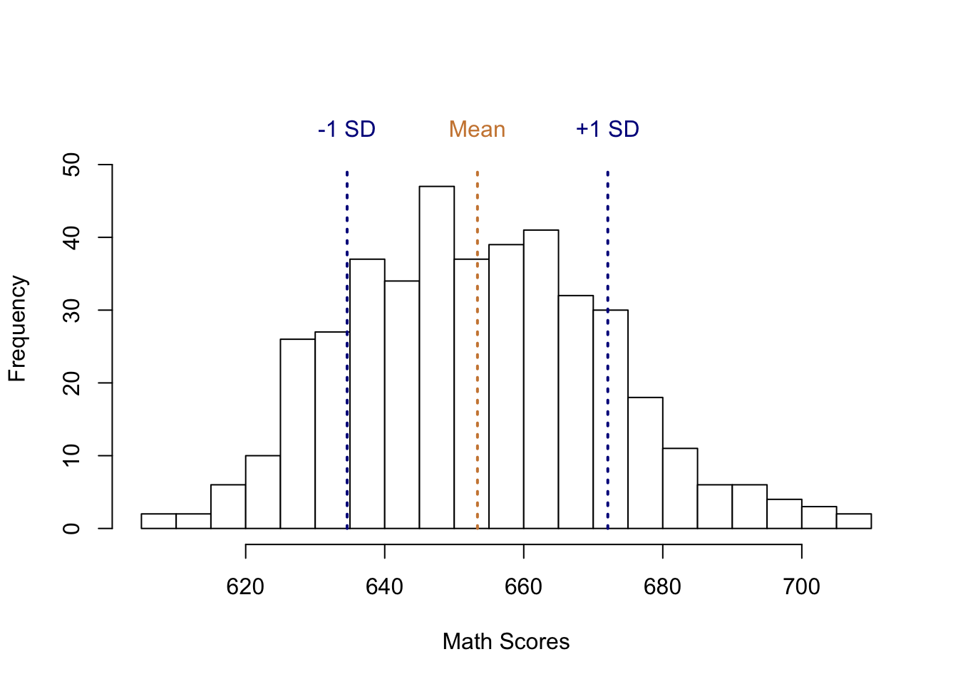
With the range set by the two blue lines falls most of our data. We would generally say that schools between the blue lines were close to average. Some were above, some where below, but that’s the sort of variation we’re willing to attribute to random chance. The school that did 1 point below the average and one point above the average aren’t considered fundamentally different, they just did a little better or worse than each other. Data does fall outside that range though, and what that indicates is that those schools did atypically well or poorly on the test.
To calculate the standard deviation by hand we need to:
- Calculate the mean
- Subtract each individual observation from the mean, and square the result
- Calculate the mean of the squared differences.
- Calculate the square root of each figure.
That’s a mouth full. We’ll see below that we can calculate standard deviation with only a few keystrokes in R
Which is to say, that calculating standard deviation is not the important lesson here. What matters is understanding what it is telling you about the data.
Let’s say you’re going to a basketball game, and the best players on both teams average around 25 points. But the standard deviation in their scoring is quite different.
| Name | Points | Standard Deviation |
|---|---|---|
| Smith | 25.12 | 3 |
| Jones | 25.28 | 12 |
Which player should you be more confident will score close to 25 points at the game? Smith. She has a much smaller standard deviation, so you can be confident that at a typical game she’ll score between 22 and 28 points. Jones runs hot or cold; they might score 37, but they could just as easily score 13. There’s a lot more variation in her games.
10.1.2.7 Summary
This chapter has worked through a lot of terminology. Means, Medians, and Modes, along with Mins and Maxs, and lets not forget percentiles or standard deviation. Actually, let’s not forget any of it. All of the terms we’ve covered in this chapter will come up again as we work into more and more of the statistics researchers use to explain the world.
But they’re also important on their own. Whenever you collect or use data, it’s important that you give the reader some summary statistics like the ones we outlined above so that they can begin to understand what you’re working with. Even if you use a common data source, like the US Census, I wont know exactly what that data looks like unless you tell me about it. So before we get to the practice of calculating or outputting descriptive statistics, let’s look at the descriptive statistics used in a few journal articles.
What we’re really talking about is a descriptive statistics table. A table that lists the variables you’re using or are important in your study, and some brief descriptive statistics (like the ones described above) so that the reader gets a better understanding of your data.
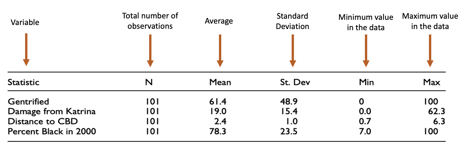
That was from a quantaititve study I did with a colleague where we looked at whether poor neighborhoods damaged by Hurricane Katrina were more or less likely to gentrify over the decade that followed. So the line for Gentrified shows that 61.4% of the 101 neighborhoods we studied did gentrify. Damage from Katrina measures the percentage of all housing in each neighborhood that was damaged by Hurricane Katrina. So the data shows that the average neighborhood had 19% of its housing damaged, but the lowest amount was 0 percent and the largest amount was 62.3% The distance to the CBD (Central Business District, or downtown) shows that the average neighborhood in our sample of 101 was 2.4 miles from downtown, with the furthest neighborhood being 6.3 miles away. Looking at the standard deviation, you can see that most neighborhoods were between 1.4 and 3.4 miles from downtown. The percentage of residents that were black in 2000 shows that the average neighborhood in our study was 78.3% black, with a range of 7% to 100%. That data is much more spread out, so the standard deviation is 23.5. 78.3 + 23.5 equals 101.8, which isn’t possible (no neighborhood can be more than 100% anything), and that’s okay for the standard deviation, the values don’t necessarily have to be meaningful in that case they’re just necessary to indicate how spread out the data is.
You’ll see descriptive statistics used in qualitative research too. Wait, you might say, qualitative research focuses on words - why would you present the average of something? So that the reader can understand who your average or typical respondent was. See the table below from the article More Than An Eyesore by Garvin and coauthors. It’s good for me to know that their sample was 59% male, typically unmarried, all Black, etc. Numbers like those are easier to read in the form of a table than writing them out, and they provide important context for your results.
10.2 Practice
So now that we are starting to understand the numbers that go into a descriptive statistics table, and we’ve seen a few examples, let’s make one ourselves. Again, we’re not going to spend a lot of time on calculating things, because R wants to do those things for us.
Let’s start by just calculating some of the statistics we have above just using R. Of course, we’ll need some data to calculate these things, so be sure to load the data on California Schools that I’m using to practice. You can copy that line of code into an R script to run it.
CASchools <- read.csv("https://raw.githubusercontent.com/ejvanholm/DataProjects/master/CASchools.csv") ## Loading in the data
head(CASchools)
## X district school county grades students
## 1 1 75119 Sunol Glen Unified Alameda KK-08 195
## 2 2 61499 Manzanita Elementary Butte KK-08 240
## 3 3 61549 Thermalito Union Elementary Butte KK-08 1550
## 4 4 61457 Golden Feather Union Elementary Butte KK-08 243
## 5 5 61523 Palermo Union Elementary Butte KK-08 1335
## 6 6 62042 Burrel Union Elementary Fresno KK-08 137
## teachers calworks lunch computer expenditure income english read
## 1 10.90 0.5102 2.0408 67 6384.911 22.690001 0.000000 691.6
## 2 11.15 15.4167 47.9167 101 5099.381 9.824000 4.583333 660.5
## 3 82.90 55.0323 76.3226 169 5501.955 8.978000 30.000002 636.3
## 4 14.00 36.4754 77.0492 85 7101.831 8.978000 0.000000 651.9
## 5 71.50 33.1086 78.4270 171 5235.988 9.080333 13.857677 641.8
## 6 6.40 12.3188 86.9565 25 5580.147 10.415000 12.408759 605.7
## math
## 1 690.0
## 2 661.9
## 3 650.9
## 4 643.5
## 5 639.9
## 6 605.4Let’s calculate the mean and median score on the reading test (since we’ve already spent so much time talking about math). R tries to keep its commands fairly basic and easy to understand, so to calculate mean you use mean() and for median you use median().
## [1] 654.9705## [1] 655.75The mean is 654.9705 and the median is 655.75, those are pretty similar numbers, so we could probably report either one if we wanted to.
We can calculate the min and the max with (drum roll)… the commands min() and max().
## [1] 604.5## [1] 704And to calculate the standard deviation we can skip those four steps described above and use the command sd().
## [1] 20.10798The standard deviation is roughly 20, meaning that most schools scored 654 on the reading test, plus or minus 20 points.
Those are all statistics that you might see in a descriptive statistics table. You could run all of those commands for all of the variables you’re interested in and build a table by hand by copying and pasting the output into the table.
Or, you can have R work on building the table for you. The summary() command will actually give you a whole set of summary statistics with just one line of code.
##    Min. 1st Qu.  Median    Mean 3rd Qu.    Max.
##   604.5   640.4   655.8   655.0   668.7   704.0
Let’s say I want descriptive statistics for more than one column in my data. The summary() command can do that, it can also produce statistics for an entire data set at once.
##        X            district                           school
##  Min.   :  1.0   Min.   :61382   Lakeside Union Elementary:  3
##  1st Qu.:105.8   1st Qu.:64308   Mountain View Elementary :  3
##  Median :210.5   Median :67760   Jefferson Elementary     :  2
##  Mean   :210.5   Mean   :67473   Liberty Elementary       :  2
##  3rd Qu.:315.2   3rd Qu.:70419   Ocean View Elementary    :  2
##  Max.   :420.0   Max.   :75440   Pacific Union Elementary :  2
##                                  (Other)                  :406
##          county      grades       students          teachers
##  Sonoma     : 29   KK-06: 61   Min.   :   81.0   Min.   :   4.85
##  Kern       : 27   KK-08:359   1st Qu.:  379.0   1st Qu.:  19.66
##  Los Angeles: 27               Median :  950.5   Median :  48.56
##  Tulare     : 24               Mean   : 2628.8   Mean   : 129.07
##  San Diego  : 21               3rd Qu.: 3008.0   3rd Qu.: 146.35
##  Santa Clara: 20               Max.   :27176.0   Max.   :1429.00
##  (Other)    :272
##     calworks          lunch           computer       expenditure
##  Min.   : 0.000   Min.   :  0.00   Min.   :   0.0   Min.   :3926
##  1st Qu.: 4.395   1st Qu.: 23.28   1st Qu.:  46.0   1st Qu.:4906
##  Median :10.520   Median : 41.75   Median : 117.5   Median :5215
##  Mean   :13.246   Mean   : 44.71   Mean   : 303.4   Mean   :5312
##  3rd Qu.:18.981   3rd Qu.: 66.86   3rd Qu.: 375.2   3rd Qu.:5601
##  Max.   :78.994   Max.   :100.00   Max.   :3324.0   Max.   :7712
##
##      income          english            read            math
##  Min.   : 5.335   Min.   : 0.000   Min.   :604.5   Min.   :605.4
##  1st Qu.:10.639   1st Qu.: 1.941   1st Qu.:640.4   1st Qu.:639.4
##  Median :13.728   Median : 8.778   Median :655.8   Median :652.5
##  Mean   :15.317   Mean   :15.768   Mean   :655.0   Mean   :653.3
##  3rd Qu.:17.629   3rd Qu.:22.970   3rd Qu.:668.7   3rd Qu.:665.9
##  Max.   :55.328   Max.   :85.540   Max.   :704.0   Max.   :709.5
##
That gets a little messier to read though.
Okay here are the more advanced lessons though. Above I just produced the descriptive statistics for all 15 variables in my data set. But maybe I don’t want all 15. Maybe I just want a few of the columns. I can create a new data set in R, just with the columns I actually want. Let’s say my analysis is focused on the math (math) and reading (read) scores for schools, along with the number of students (students) and the median income of parents (income). I can select those columns by name, as I do below.
##    read  math students    income
## 1 691.6 690.0      195 22.690001
## 2 660.5 661.9      240  9.824000
## 3 636.3 650.9     1550  8.978000
## 4 651.9 643.5      243  8.978000
## 5 641.8 639.9     1335  9.080333
## 6 605.7 605.4      137 10.415000
I’m going to break that down in detail here, but it may not still completely make sense until you practice it 100 times. I figured out that line of code by googling “how to select columns by name” dozens of times until I learned the way to do it. I’d find some post online that had the answer, and just copy the code and change the names to match my data. That’s most of what learning to code is all about. But anyways, the explanation:
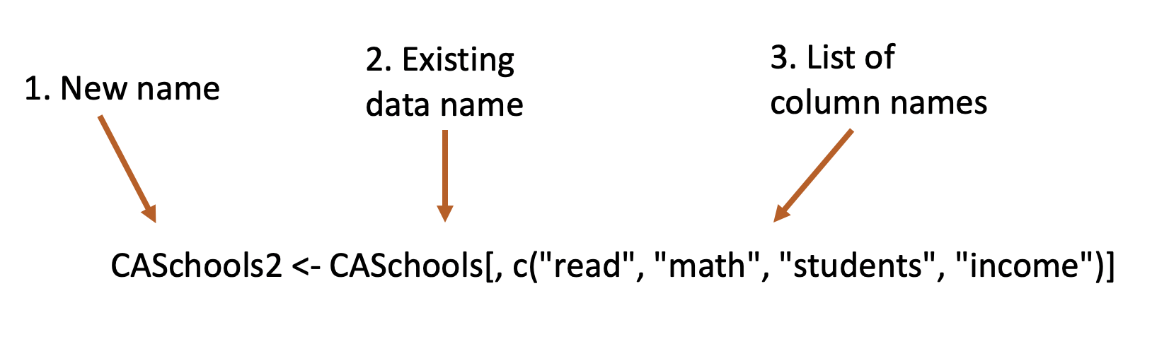
What this line of code is saying overall is look in this object called CASchools, find the columns names read, math, students, and income, and make that into a new object called CASchools2.
New name. I’m creating a new object here called CASchools2. That way I’ll have the old data set CASchools still in my environment with all the columns, but also have a new data set called CASchools2 with just the 4 columns I want. I could name it anything I want, but I choose the name CASchools2 so that it would be similar to the original data, but the “2” is added so I know it is a different version.
I need to tell R what data I’m taking the columns from, so i need to identify CASchools by name.
I then tell R the list of variables I want from CASchools. To make a list I need to include the c outside the parenthesis, similar to how we created an object called y with the values 1,2,3 in the last chapter. So I’m saying this list of 4 columns that are in CASchools.
This would be a really good time to practice that line of code, and try to extract the columns “lunch”, “computer”, “expenditure”, “income”, or some other list. Remember, to look up all the column names in a data set you can use the command names(). It’d also be a good idea to change the name of the new object, try any word you want instead of CASchools2. Change everything until the code gives you an error message, and then go back a step to something that worked.
Okay, but for now we’ve got fewer columns in our data frame called CASchools2, so there will be less text in our summary statistics.
##       read            math          students           income
##  Min.   :604.5   Min.   :605.4   Min.   :   81.0   Min.   : 5.335
##  1st Qu.:640.4   1st Qu.:639.4   1st Qu.:  379.0   1st Qu.:10.639
##  Median :655.8   Median :652.5   Median :  950.5   Median :13.728
##  Mean   :655.0   Mean   :653.3   Mean   : 2628.8   Mean   :15.317
##  3rd Qu.:668.7   3rd Qu.:665.9   3rd Qu.: 3008.0   3rd Qu.:17.629
##  Max.   :704.0   Max.   :709.5   Max.   :27176.0   Max.   :55.328
10.2.1 Advanced Practice
Anyone not interested in continuing to practice their coding skills can get off the bus here. It’ll move a little faster (less explanation), and these exercises are more meant for people that are actively looking to see the full potential of using R in a project.
You can copy the output of a table produced by summary() and put it in a word document, but below I’m going to give you some more code to show how I actually build a descriptive statistics table for one of my papers.
With a few more steps though you can A) select the exact statistics you want for your summary table and B) add the standard deviation.
Fair warning: There might be a better or more efficient way to produce what I do below. In fact, there probably is. If you can improve on it, great! Please tell me how. I’m really bad at using loops, so that might improve this code, but I’m not sure where to start and just reusing this code makes it quicker than learning how to improve it.
First I create a new data frame using the command as.data.frame() with a list of the names of variables I want. I don’t use the short descriptions I have for column names in the data, but rather a more informative title that will start to tell the reader what the data is. I’ll use the same 4 variables we have in CASchools2 above.
# creating new data frame called name with names of variables

names <- as.data.frame(c( "Reading Test Scores",
                         "Math Test Scores",
                         "Number of Students",
                         "Median Income of Parents"))
And I’m going to rename the column in that data frame using colnames() as “Variables” so that I know exactly what it holds.
##                  Variables
## 1      Reading Test Scores
## 2         Math Test Scores
## 3       Number of Students
## 4 Median Income of Parents
I then generate a separate object for each variable with the summary statistics saved. I’ll name those x1, x2, x3, x4 as a very simple name that tells me the order I created them.
# creating new data frame called name with names of variables

x1 <- summary(CASchools2$read)
x2 <- summary(CASchools2$math)
x3 <- summary(CASchools2$students)
x4 <- summary(CASchools2$income)
Just to show you what that did, let’s look at object x1. It just has the same summary statistics we produced above for the variable read.
##    Min. 1st Qu.  Median    Mean 3rd Qu.    Max.
##   604.5   640.4   655.8   655.0   668.7   704.0
By saving it as an object we can now select the elements in we want from that list. The default summary statistics in R has 6 figures (min, 1st quartile, median, mean, 3rd quartile, and max) but we may not want to show all of those all the time.
First we combine the 4 different objects x1, x2, x3, and x4 with the command rbind(), which stands for rbind.
##       Min. 1st Qu.   Median       Mean  3rd Qu.      Max.
## x1 604.500 640.400 655.7500  654.97048  668.725   704.000
## x2 605.400 639.375 652.4500  653.34262  665.850   709.500
## x3  81.000 379.000 950.5000 2628.79286 3008.000 27176.000
## x4   5.335  10.639  13.7278   15.31659   17.629    55.328
Then we select only the columns we want. Specifically, I’d like to keep the mean, min, and max and I’ll place those three columns in a new object called s (for summary).
##          Mean    Min.      Max.
## x1  654.97048 604.500   704.000
## x2  653.34262 605.400   709.500
## x3 2628.79286  81.000 27176.000
## x4   15.31659   5.335    55.328
Great, now the object s only has the 3 columns I wanted. Earlier I combined different rows of data with the command rbind(). Now I’ll combine different columns with cbind(), specifically the column of variable names we created earlier (names) and the 3 columns of summary statistics in s.
##                   Variables       Mean    Min.      Max.
## x1      Reading Test Scores  654.97048 604.500   704.000
## x2         Math Test Scores  653.34262 605.400   709.500
## x3       Number of Students 2628.79286  81.000 27176.000
## x4 Median Income of Parents   15.31659   5.335    55.328
Two more steps to go. Now I’m going to generate the standard deviation for each variable, which isn’t included in the default summary statistics table. and I’ll save that as an object named sd and give it the column name “SD”.
# generating standard deviations for all 4 variables

sd <- as.data.frame(c( sd(CASchools2$read, na.rm=TRUE),
                       sd(CASchools2$math, na.rm=TRUE),
                       sd(CASchools2$students, na.rm=TRUE),
                       sd(CASchools2$income, na.rm=TRUE)  ))
colnames(sd) <- "SD"
sd
## SD
## 1 20.10798
## 2 18.75420
## 3 3913.10498
## 4 7.22589And then we add that new column to our existing data frame called s, and we’re done.
##                   Variables       Mean    Min.      Max.         SD
## x1      Reading Test Scores  654.97048 604.500   704.000   20.10798
## x2         Math Test Scores  653.34262 605.400   709.500   18.75420
## x3       Number of Students 2628.79286  81.000 27176.000 3913.10498
## x4 Median Income of Parents   15.31659   5.335    55.328    7.22589
That is closer to the type of summary statistics table that I would use in a paper. I might also round all of the figures, as a final step. I’ll let the decimals show one digit using the command round() by entering the name of the column followed by a comma and the number 1. If I wanted no decimals I could use the number 0, or if I wanted 2 decimal places I could use 2.
# rounding numbers in a column

s3$Mean <- round(s3$Mean,1)
s3$Min <- round(s3$Min,1)
s3$Max <- round(s3$Max,1)
s3$SD <- round(s3$SD,1)
s3
## Variables Mean Min. Max. SD Min Max
## x1 Reading Test Scores 655.0 604.500 704.000 20.1 604.5 704.0
## x2 Math Test Scores 653.3 605.400 709.500 18.8 605.4 709.5
## x3 Number of Students 2628.8 81.000 27176.000 3913.1 81.0 27176.0
## x4 Median Income of Parents 15.3 5.335 55.328 7.2 5.3 55.3If I click on the object s3 or write the command View(s3) I can copy and paste that output into my word document for final formatting. Or I could write it into an excel document, but that is for another lesson.