10 Seminar Nine

In the lecture this week you will have learnt about quantitative analysis. In this session you will perform some data analysis of your own using the mini study data sets from earlier in the module. Then you will use your new statistical knowledge to analyse the data you have collected as part of your experimental trial.

There are many statistical analysis software packages available, including SPSS, R, Python, Matlab, Jamovi, and JASP. We will be using the JAMOVI Cloud to perform all of our data analysis.

The following resources are available to help you navigate and use Jamovi

10.1 Task 1

We will use the mini_study_react to better understand how to generate descriptive statistics.

Open the mini study reaction time dataset file and save it to your own onedrive account. Now open it in Jamovi (Menu | Open | This Device | ‘file_path’)

We will start by using descriptive statistics to describe the characteristics of the participant in the study. This will allow a reader to evaluate the internal validity (the extent to which the observed results represent the truth in the population we are studying) and external validity (the extent to which you can generalise the findings of a study to other situations, people, settings, and measures outside of the study).

The following video is a useful guide to performing descriptive statistics in Jamovi: Descriptive Statistics Tutorial

10.1.1 Descriptive Statistic Instructions

First, lets start by describing everyone in the dataset in its entirety.

Navigate to the Exploration icon and select Descriptives
Select the variables you want to generate descriptive statistics for (Age, Weight, Height, BMI) and transfer them into the variables box
This will automatically generate a table with the descriptive statistics in the output window
The defaults are N, missing, mean, median, standard deviation, minimum, maximum
As we previously discussed not all of these are necessary, for the purposes of this task we only want to report N, mean, standard deviation
Using the statistics drop down menu to select and deselect the variables you want to present
NB You can also choose to display the variable outputs across rows or columns

Now, lets describe participants according to which group/arm they were allocated. This will allow us/the reader to evaluate whether the groups were similar at baseline

Navigate to the Exploration icon and select Descriptives
Select the variables you want to generate descriptive statistics for (Age, Weight, Height, BMI) and transfer them into the variables box
This will automatically generate a table with the descriptive statistics in the output window
Now select the variable that indicates which group participants were assigned to (allocation) and transfer it to the ‘split by’ box
- This will automatically generate a table with the descriptive statistics for each group/arm in the output window
The defaults are N, missing, mean, median, standard deviation, minimum, maximum
As we previously discussed not all of these are necessary, for the purposes of this task we only want to report N, mean, standard deviation
Using the statistics drop down menu to select and deselect the variables you want to present
NB You can also choose to display the variable outputs across rows or columns

The data outputs generated are generally formatted correctly for APA presentation and can be exported/copied and pasted directly into your manuscripts or presentations. Simply right click the table and choose your option

10.2 Task 2

Using the instructions above, generate the descriptive statistics for your own dataset. You Should include a descriptive statistics table in your academic poster (assessment).

10.3 Task 3

10.3.1 Descriptive statistics for the outcome(s) of interest

The next step is to generate descriptive statistics on the outcomes that were measured in the study.

We will use the mini_study_KTW to better understand how to generate descriptive statistics for the outcome of interest.

Open the mini study knee to wall dataset file and save it to your own onedrive account. Now open it in Jamovi (Menu | Open | This Device | ‘file_path’)

Navigate to the Exploration icon and select Descriptives
Select the variables you want to generate descriptive statistics for (pre_range, post_range) and transfer them into the variables box
This will automatically generate a table with the descriptive statistics in the output window
The defaults are N, missing, mean, median, standard deviation, minimum, maximum
As we previously discussed not all of these are necessary, for the purposes of this task we only want to report N, mean, standard deviation
Using the statistics drop down menu to select and deselect the variables you want to present
NB You can also choose to display the variable outputs across rows or columns

Now we have explored the data we can perform inferential statistics to determine whether the difference observed between the two (or more) groups is statistically significant (ie the probability of the null hypothesis being true compared to the acceptable level of uncertainty regarding the true answer).

10.3.2 Selecting the correct statistical test

Before we can do this we need to identify which statistical approach is best and check that the data meets the statistical assumptions for that test.

Use the image below to identify what the correct statistical test is for analysing whether there is a mean difference in ankle range of movement within participants in this non-randomised, unblinded, single arm, pre-test post-test study.

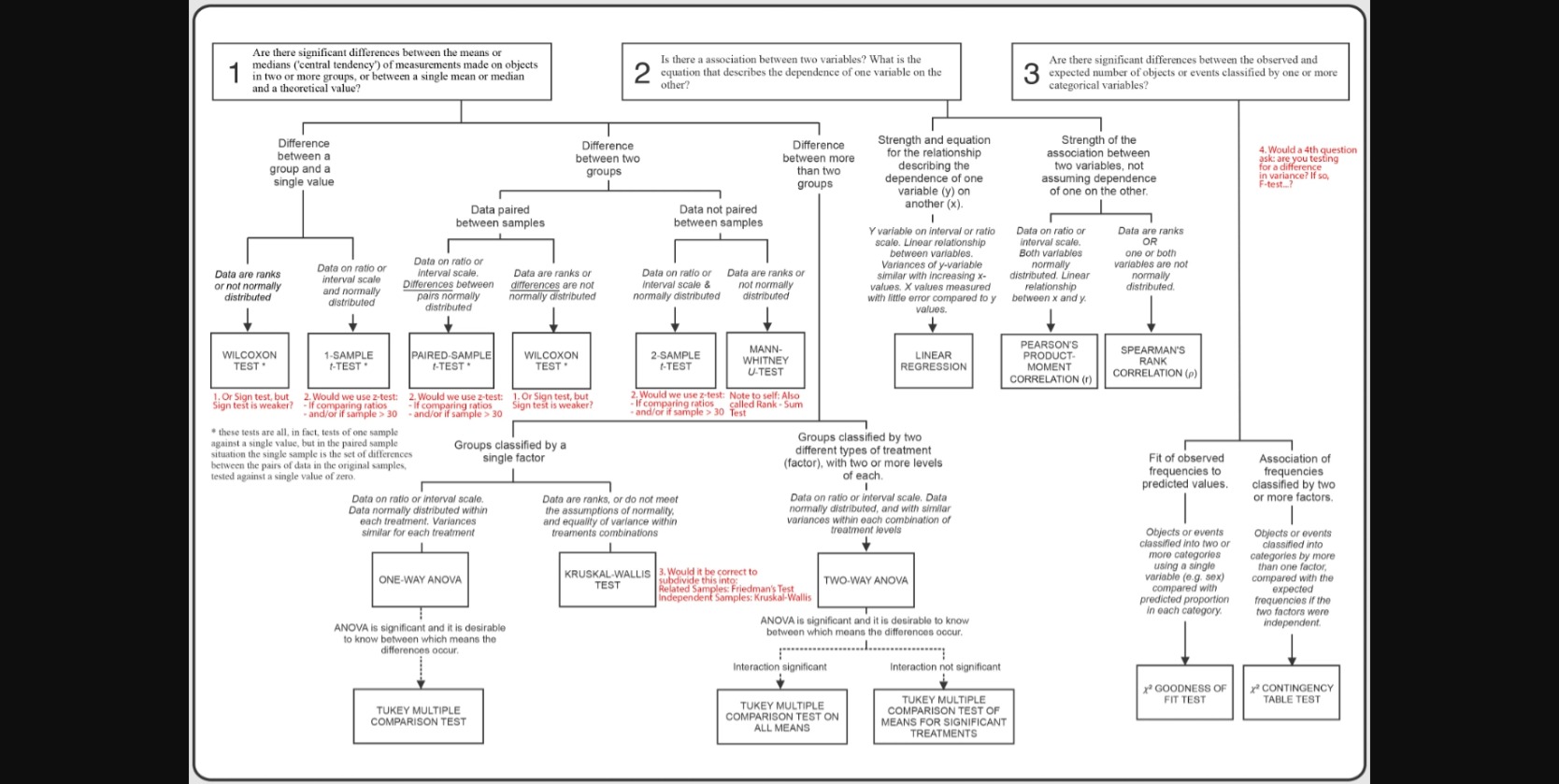
Hopefully, you reached the conclusion that a paired t-test is the statistical test of choice

The following video is a useful guide to performing a paired t-test in Jamovi: Paired T-test tutorial

A paired T-test assumes the following three things:

Independence: Each observation should be independent of every other observation
Normality: The differences between the pairs should be approximately normally distributed
No Extreme Outliers: There should be no extreme outliers in the differences

10.3.3 Conducting a paired T-Test

Open the mini study knee to wall dataset file and save it to your own onedrive account. Now open it in Jamovi (Menu | Open | This Device | ‘file_path’)

Navigate to the T-Tests icon and select Paired Samples T-Test
Select the two variables you want to compare (pre_range, post_range) and transfer them into the paired variables box
This will automatically generate a table with the inferential statistics in the output window
The defaults are statistic, df, p value
If the p value is <0.05 the null hypothesis can be rejected and the mean difference observed is unlikely due to chance (therefore the intervention is likely to have caused the change in scores)
It is often helpful to also include the mean difference, descriptives and descriptives plot
We can also select normality to check that the normality assumption is met (NB if the p value is <0.05 the assumption has been violated and a wilcoxon rank test is more suitable)

10.4 Task 4

We will use the mini_study_pap to demonstrate a different statistical test.

Open the [mini study post activation potentiation and save it to your own onedrive account. Now open it in Jamovi (Menu | Open | This Device | ‘file_path’)

Using what you have learnt so far produce the descriptive statistics for the outcomes of this study

Use the image below to identify what the correct statistical test is for comparing the mean difference between participants in this randomised, unblinded, parallel two-arm study.

Hopefully, you reached the conclusion that an independent t-test is the statistical test of choice

An independent samples T-Test assumes the following:

The dependent variable is measured on a continuous scale
The independent variable consists of two categorical, independent groups
There is no relationship between the observations in each group or between the groups themselves
There should be no significant outliers
The dependent variable should be approximately normally distributed for each group of the independent variable
There needs to be homogeneity of variances

10.4.1 Conducting an independent T-Test

The following video is a useful guide to performing an independent t-test in Jamovi: Independent T-test tutorial

Navigate to the T-Tests icon and select Indepedent Samples T-Test
Select the variable(s) you want to compare (cmj_height_mean, cmj_flight_mean) and transfer them into the dependent variables box
Now select the variable that indicates which group participants were assigned to (allocation) and transfer it to the ‘grouping variable’ box
This will automatically generate a table with the inferential statistics in the output window
The defaults are statistic, df, p value
If the p value is <0.05 the null hypothesis can be rejected and the mean difference observed is unlikely due to chance (therefore the intervention is likely to have caused the change in scores)
It is often helpful to also include the mean difference, descriptives and descriptives plot
We can also select homogeneity and normality to check that the homogeneity and normality assumptions are met (NB if the p value is <0.05 the assumption has been violated and a Mann Whitney U test is more suitable)

10.5 Task 5

Finally, lets analyse the last of our mini study series.

We will use the mini_study_react to demonstrate a different statistical test.

Open the mini study reaction time dataset file and save it to your own onedrive account. Now open it in Jamovi (Menu | Open | This Device | ‘file_path’)

Using what you have learnt so far produce the descriptive statistics for the outcomes of this study

Use the the image below to identify what the correct statistical test is for comparing the mean difference between participants in this randomised, unblinded, parallel three-arm study.

Hopefully, you reached the conclusion that a one-way ANOVA is the statistical test of choice

A one-way ANOVA assumes the following:

The dependent variable is measured at the interval or ratio level (i.e., they are continuous)
The independent variable should consist of two or more categorical, independent groups
There is no relationship between the observations in each group or between the groups themselves
There are no significant outliers
The dependent variable should be approximately normally distributed for each category of the independent variable
There needs to be homogeneity of variances

10.5.1 Conducting a one-way ANOVA

The following video is a useful guide to performing an one-way ANOVA in Jamovi: one-way ANOVA tutorial

Navigate to the ANOVA icon and select One-way T-Test
Select the variable(s) you want to compare (post_reaction_time) and transfer them into the dependent variables box
Now select the variable that indicates which group participants were assigned to (allocation) and transfer it to the ‘grouping variable’ box
This will automatically generate a table with the inferential statistics in the output window
The defaults are F statistic, df1, df2, p value
If the p value is <0.05 the null hypothesis can be rejected and the mean difference observed is unlikely due to chance (therefore the intervention is likely to have caused the change in scores)
It is often helpful to also include descriptives and descriptives plot
We can also select homogeneity and normality to check that the homogeneity and normality assumptions are met
If the p value for the one-way ANOVA is <0.05, further analysis is needed to identify which comparison(s) where considered significantly different. This further analysis is known as post hoc testing
Although, the one-way analysis was not significant (p=0.251) lets perform the post hoc analysis to demonstrate the procedure
Open the Post-Hoc Test dialogue box and choose the Tukey (equal variance) comparison
Review the post hoc output for the individual group comparisons

10.6 Task 6

Using the what you have learnt so far,identify the relevant statistical test for your study and perform the statistical analysis. You Should include the relevant statistical output in your academic poster (assessment).

9 Seminar Eight

11 Seminar Ten