Chapter 2 Working with Data (FQA)
This section provides an overview of useful commands for working with tabular data in R.
2.1 Reading in Data
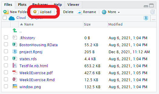
2.1.1 Uploading Data to RStudio Cloud
To read in data from a file, that file must be stored in the RStudio Cloud project you are working within. Typically, the data files you need will come pre-loaded in the projects we share with you. However, if you need to upload your own data file, you can do so by clicking the “Upload” button in the bottom-right pane of RStudio (see image below).
2.1.2 Reading in CSV Files
Throughout HBAP we will typically work with data stored in comma-separated value (.csv) files. Once a file is loaded into your RStudio Cloud project, you can read it in with the read.csv() function. The file name you pass into the function must be surrounded by quotation marks ("").
##     ID                Name Gender Age Rating      Degree Start_Date Retired
## 1 6881  al-Rahimi, Tayyiba Female  51     10 High School  2/23/1990   FALSE
## 2 2671       Lewis, Austin   Male  34      4        Ph.D  2/23/2007   FALSE
## 3 8925   el-Jaffer, Manaal Female  50     10    Master's  2/23/1991   FALSE
## 4 2769       Soto, Michael   Male  52     10 High School  2/23/1987   FALSE
## 5 2658 al-Ebrahimi, Mamoon   Male  55      8        Ph.D  2/23/1985   FALSE
## 6 1933      Medina, Brandy Female  62      7 Associate's  2/23/1979    TRUE
##      Division Salary
## 1  Operations 108804
## 2 Engineering 182343
## 3 Engineering 206770
## 4       Sales 183407
## 5   Corporate 236240
## 6       Sales     NA
2.2 Data Frame Basics
We can count the number of observations (or rows) in our data set with nrow():
## [1] 1000Similarly, we can count the number of variables (or columns) with ncol():
## [1] 10We can get a list of the variable names with names():
##  [1] "ID"         "Name"       "Gender"     "Age"        "Rating"
##  [6] "Degree"     "Start_Date" "Retired"    "Division"   "Salary"
We can access specific columns in our data set with the $ operator. For example, the code below calculates the average age in our data set.
## [1] 45.53The str() command prints out the structure of the data, which indicates the recognized type of each variable:
## 'data.frame':    1000 obs. of  10 variables:
##  $ ID        : int  6881 2671 8925 2769 2658 1933 3570 7821 3256 6222 ...
##  $ Name      : chr  "al-Rahimi, Tayyiba" "Lewis, Austin" "el-Jaffer, Manaal" "Soto, Michael" ...
##  $ Gender    : chr  "Female" "Male" "Female" "Male" ...
##  $ Age       : int  51 34 50 52 55 62 47 43 27 30 ...
##  $ Rating    : int  10 4 10 10 8 7 8 8 7 6 ...
##  $ Degree    : chr  "High School" "Ph.D" "Master's" "High School" ...
##  $ Start_Date: chr  "2/23/1990" "2/23/2007" "2/23/1991" "2/23/1987" ...
##  $ Retired   : logi  FALSE FALSE FALSE FALSE FALSE TRUE ...
##  $ Division  : chr  "Operations" "Engineering" "Engineering" "Sales" ...
##  $ Salary    : int  108804 182343 206770 183407 236240 NA 101138 149468 74188 110078 ...
Finally, the summary() command provides an intelligent summary of each variable in the data set, based on the variable’s type:
##        ID           Name              Gender               Age
##  Min.   :1030   Length:1000        Length:1000        Min.   :25.00
##  1st Qu.:3225   Class :character   Class :character   1st Qu.:36.00
##  Median :5360   Mode  :character   Mode  :character   Median :46.00
##  Mean   :5384                                         Mean   :45.53
##  3rd Qu.:7496                                         3rd Qu.:56.00
##  Max.   :9973                                         Max.   :65.00
##
##      Rating          Degree           Start_Date         Retired
##  Min.   : 2.000   Length:1000        Length:1000        Mode :logical
##  1st Qu.: 6.000   Class :character   Class :character   FALSE:920
##  Median : 7.000   Mode  :character   Mode  :character   TRUE :80
##  Mean   : 6.993
##  3rd Qu.: 8.000
##  Max.   :10.000
##
##    Division             Salary
##  Length:1000        Min.   : 29825
##  Class :character   1st Qu.:129694
##  Mode  :character   Median :156290
##                     Mean   :156486
##                     3rd Qu.:184742
##                     Max.   :266235
##                     NA's   :80
2.3 Manipulating Data Frames
2.3.1 Subsetting Data
There are two ways to subset a data set. One method is to use the subset() function, where the first argument is the data frame and the second is the filtering condition. For example, the code below creates a new data frame called dataHighPerformers with only those employees whose Rating is greater than or equal to 8.
##     ID                 Name Gender Age Rating      Degree Start_Date Retired
## 1 6881   al-Rahimi, Tayyiba Female  51     10 High School  2/23/1990   FALSE
## 3 8925    el-Jaffer, Manaal Female  50     10    Master's  2/23/1991   FALSE
## 4 2769        Soto, Michael   Male  52     10 High School  2/23/1987   FALSE
## 5 2658  al-Ebrahimi, Mamoon   Male  55      8        Ph.D  2/23/1985   FALSE
## 7 3570  Troftgruben, Tierra Female  47      8 High School  2/23/1995   FALSE
## 8 7821 Holleman, Shaquaisha Female  43      8    Master's  2/23/1999   FALSE
##          Division Salary
## 1      Operations 108804
## 3     Engineering 206770
## 4           Sales 183407
## 5       Corporate 236240
## 7      Operations 101138
## 8 Human Resources 149468
Alternatively, we can specify the condition within brackets. Within the brackets, the first position indicates the rows we want to extract, which in this case is all rows where Rating is greater than or equal to 8. The second position indicates the columns we want to extract; we can extract all columns by leaving this position empty.
##     ID                 Name Gender Age Rating      Degree Start_Date Retired
## 1 6881   al-Rahimi, Tayyiba Female  51     10 High School  2/23/1990   FALSE
## 3 8925    el-Jaffer, Manaal Female  50     10    Master's  2/23/1991   FALSE
## 4 2769        Soto, Michael   Male  52     10 High School  2/23/1987   FALSE
## 5 2658  al-Ebrahimi, Mamoon   Male  55      8        Ph.D  2/23/1985   FALSE
## 7 3570  Troftgruben, Tierra Female  47      8 High School  2/23/1995   FALSE
## 8 7821 Holleman, Shaquaisha Female  43      8    Master's  2/23/1999   FALSE
##          Division Salary
## 1      Operations 108804
## 3     Engineering 206770
## 4           Sales 183407
## 5       Corporate 236240
## 7      Operations 101138
## 8 Human Resources 149468
2.3.2 Sorting Data
You can sort data on specific columns using the order() function:
##       ID                  Name Gender Age Rating      Degree Start_Date Retired
## 12  7068          Dimas, Roman   Male  25      8 High School  2/23/2017   FALSE
## 96  5464      al-Pirani, Rajab   Male  25      3 Associate's  2/23/2016   FALSE
## 126 7910        Hopper, Summer Female  25      7  Bachelor's  2/23/2017   FALSE
## 261 6784 al-Siddique, Zaitoona Female  25      4    Master's  2/23/2015   FALSE
## 322 3240        Steggall, Shai Female  25      7    Master's  2/23/2017   FALSE
## 358 1413          Tanner, Sean   Male  25      2 Associate's  2/23/2016   FALSE
##            Division Salary
## 12       Operations  84252
## 96       Operations  37907
## 126     Engineering 100688
## 261 Human Resources 127618
## 322      Operations 117062
## 358      Operations  61869
You can reverse the direction of the sort by adding a negative sign (-) in front of the variable:
##       ID              Name Gender Age Rating      Degree Start_Date Retired
## 137 8060 al-Morad, Mastoor   Male  65      8        Ph.D  2/23/1977   FALSE
## 223 9545    Lloyd, Devante   Male  65      9  Bachelor's  2/23/1974   FALSE
## 248 7305     Law, Charisma Female  65      8 Associate's  2/23/1976   FALSE
## 295 4141  Herrera, Yarabbi Female  65      8 High School  2/23/1975   FALSE
## 340 2559     Holiday, Emma Female  65      7  Bachelor's  2/23/1975    TRUE
## 462 4407     Ross, Caitlyn Female  65      7  Bachelor's  2/23/1975    TRUE
##            Division Salary
## 137       Corporate 213381
## 223      Accounting 243326
## 248 Human Resources 214788
## 295      Operations 143728
## 340      Operations     NA
## 462       Corporate     NA
2.4 Summary Statistics
2.4.1 Quantitative Variables
We can apply all of the following functions to any quantitative variable in a data frame to calculate basic summary statistics:
mean()median()sd()summary()
## [1] 45.53## [1] 46## [1] 11.62102The summary() function outputs the mean, median, and quartiles:
##    Min. 1st Qu.  Median    Mean 3rd Qu.    Max.
##   25.00   36.00   46.00   45.53   56.00   65.00
If the column contains any missing values (NA), we need to add the optional na.rm = TRUE argument to these functions. For example:
## [1] 156486We can use the cor() function to calculate the correlation between two quantitative variables. For this function, we need to add the optional argument use = "complete.obs" if either column contains missing values (instead of the typical na.rm = TRUE).
## [1] 0.56351252.4.2 Categorical Variables
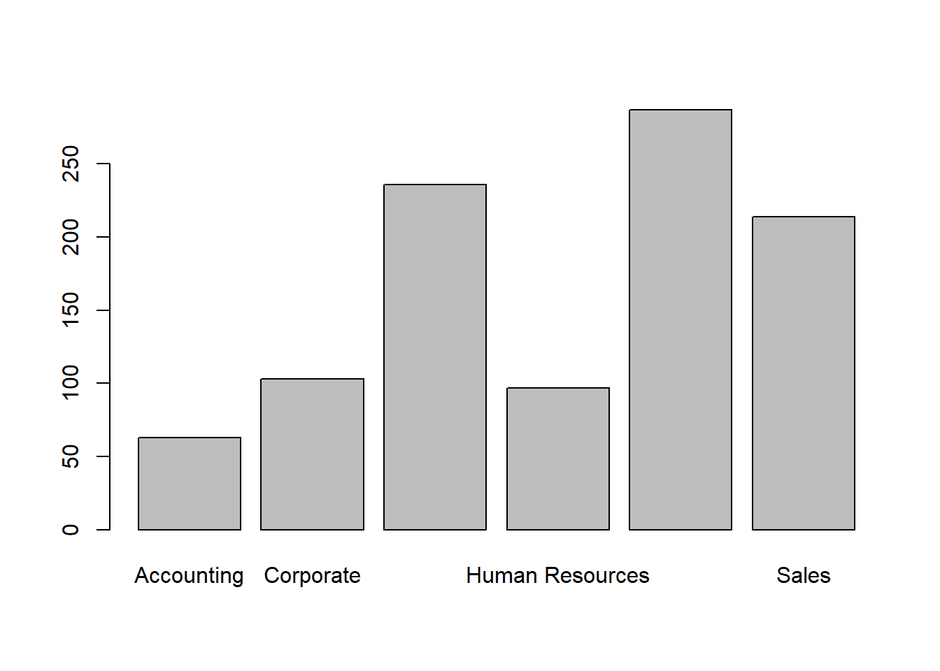
We can count the values of a categorical variable using the table() function:
##
##      Accounting       Corporate     Engineering Human Resources      Operations
##              63             103             236              97             287
##           Sales
##             214
If we want the proportion of each category (instead of the count), we need to surround our call to table() with prop.table():
##
##      Accounting       Corporate     Engineering Human Resources      Operations
##           0.063           0.103           0.236           0.097           0.287
##           Sales
##           0.214
Two categorical variables can be summarized in a two-way table using the same table() and prop.table() commands shown above. For example:
##
##                   Associate's Bachelor's High School Master's Ph.D
##   Accounting                0         31           0       32    0
##   Corporate                 0         20           0       40   43
##   Engineering               0         36           0       43  157
##   Human Resources          35         30           0       32    0
##   Operations              110         16         146       15    0
## Sales 55 67 54 38 0##
## Associate's Bachelor's High School Master's Ph.D
## Accounting 0.000 0.031 0.000 0.032 0.000
## Corporate 0.000 0.020 0.000 0.040 0.043
## Engineering 0.000 0.036 0.000 0.043 0.157
## Human Resources 0.035 0.030 0.000 0.032 0.000
## Operations 0.110 0.016 0.146 0.015 0.000
## Sales 0.055 0.067 0.054 0.038 0.000Within prop.table(), we can use the margin argument to normalize by row (margin = 1) or by column (margin = 2):
##
##                   Associate's Bachelor's High School   Master's       Ph.D
##   Accounting       0.00000000 0.49206349  0.00000000 0.50793651 0.00000000
##   Corporate        0.00000000 0.19417476  0.00000000 0.38834951 0.41747573
##   Engineering      0.00000000 0.15254237  0.00000000 0.18220339 0.66525424
##   Human Resources  0.36082474 0.30927835  0.00000000 0.32989691 0.00000000
##   Operations       0.38327526 0.05574913  0.50871080 0.05226481 0.00000000
## Sales 0.25700935 0.31308411 0.25233645 0.17757009 0.00000000##
## Associate's Bachelor's High School Master's Ph.D
## Accounting 0.000 0.155 0.000 0.160 0.000
## Corporate 0.000 0.100 0.000 0.200 0.215
## Engineering 0.000 0.180 0.000 0.215 0.785
## Human Resources 0.175 0.150 0.000 0.160 0.000
## Operations 0.550 0.080 0.730 0.075 0.000
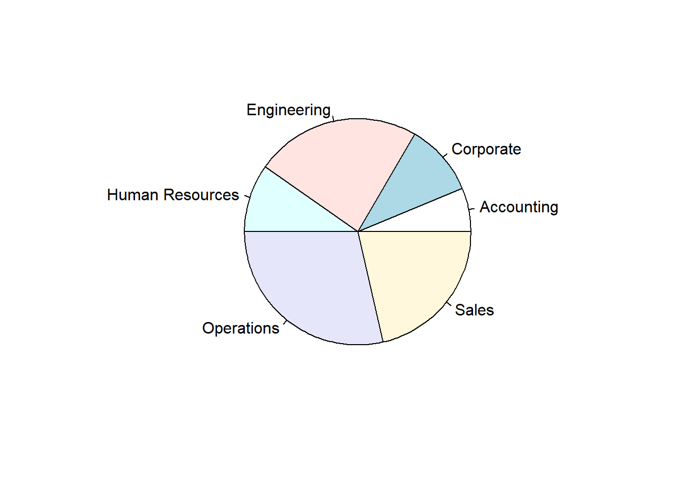
## Sales 0.275 0.335 0.270 0.190 0.0002.5 Visualizations
2.5.1 Quantitative Variables
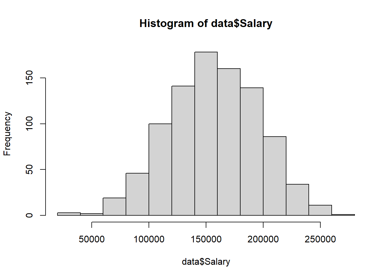
To visualize a quantitative variable we can create a histogram using the hist() function:
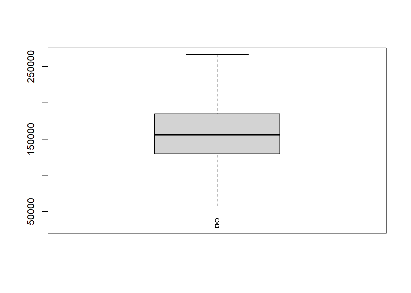
Alternatively, we can create a boxplot using the boxplot() function:
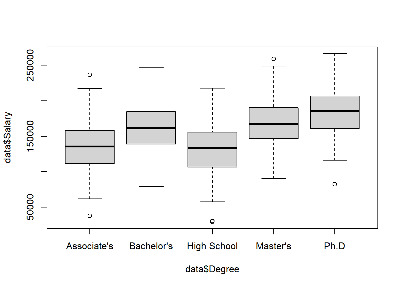
If we want to visualize the distribution of a quantitative variable over each category of a categorical variable, we can create a side-by-side boxplot. To do this we use the same boxplot() function as above, but add a tilde (~) and the categorical variable:
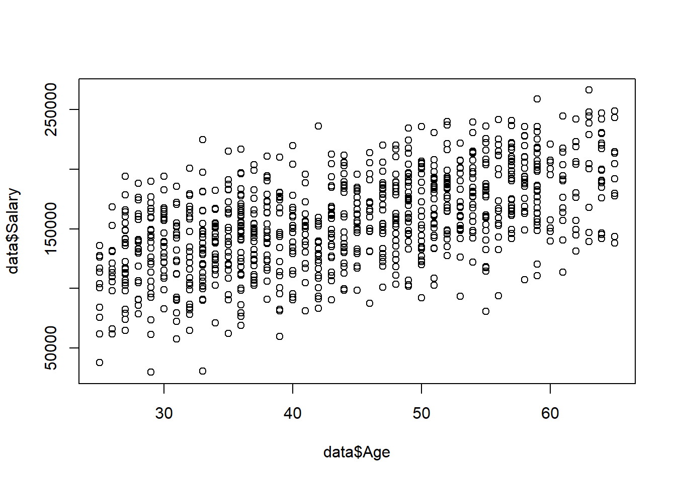
To visualize the relationship between two quantitative variables we can create a scatterplot with the plot() function: