Chapter 5 Linear Regression (FQA, OSCM)
5.1 Simple Linear Regression
Simple linear regression allows us to model a continuous variable \(Y\) as a function of a single \(X\) variable. The assumed underlying relationship is:
\[Y = \beta_{0} + \beta_{1}X + \epsilon\]
Using the method of least squares, we can estimate \(\beta_{0}\) and \(\beta_{1}\) from our sample data.
Below we use the lm() function to model the Salary variable as a function of the Age variable from data.
To view the coefficient estimates and other diagnostic information about our model, we apply the summary() function to modelSimple:
##
## Call:
## lm(formula = Salary ~ Age, data = data)
##
## Residuals:
##     Min      1Q  Median      3Q     Max
## -103272  -21766    2428   23138   90680
##
## Coefficients:
##             Estimate Std. Error t value Pr(>|t|)
## (Intercept) 67133.70    4455.17   15.07   <2e-16 ***
## Age          2026.83      98.07   20.67   <2e-16 ***
## ---
## Signif. codes:  0 '***' 0.001 '**' 0.01 '*' 0.05 '.' 0.1 ' ' 1
##
## Residual standard error: 32630 on 918 degrees of freedom
##   (80 observations deleted due to missingness)
## Multiple R-squared:  0.3175, Adjusted R-squared:  0.3168
## F-statistic: 427.1 on 1 and 918 DF,  p-value: < 2.2e-16
We can extract our estimates of the coefficients (\(\beta_{0}\) and \(\beta_{1}\)) with the coef() function.
## (Intercept)         Age
##   67133.703    2026.828
The confint() function provides a 95% confidence interval for the intercept (\(\beta_{0}\)) and slope (\(\beta_{1}\)).
##                 2.5 %    97.5 %
## (Intercept) 58390.197 75877.208
## Age          1834.364  2219.292
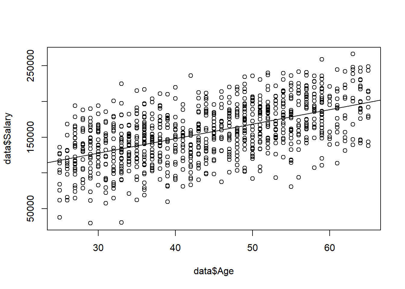
We can visualize our estimated regression line with the abline() function. First we need to create a scatterplot of Salary and Age using plot(). If we then run the abline() function on our model, it will plot the regression equation on top of the scatterplot.

5.2 Multiple Linear Regression
Multiple linear regression allows us to model a continuous variable \(Y\) as a function of multiple \(X\) variables. The assumed underlying relationship is:
\[Y = \beta_{0} + \beta_{1}X_{1} +\beta_{2}X_{2} + ... + \beta_{k}X_{k} + \epsilon\]
We use the same functions as the previous section, but now specify multiple \(X\) variables in our call to lm().
##
## Call:
## lm(formula = Salary ~ Age + Rating + Gender + Degree, data = data)
##
## Residuals:
##    Min     1Q Median     3Q    Max
## -64403 -16227    352  15917  70513
##
## Coefficients:
##                   Estimate Std. Error t value Pr(>|t|)
## (Intercept)        9481.98    4358.57   2.175 0.029850 *
## Age                2006.08      70.08  28.627  < 2e-16 ***
## Rating             5181.07     401.49  12.905  < 2e-16 ***
## GenderMale         8220.11    1532.33   5.364 1.03e-07 ***
## DegreeBachelor's  23588.25    2452.07   9.620  < 2e-16 ***
## DegreeHigh School -9477.56    2444.09  -3.878 0.000113 ***
## DegreeMaster's    31211.02    2437.29  12.806  < 2e-16 ***
## DegreePh.D        44253.05    2434.40  18.178  < 2e-16 ***
## ---
## Signif. codes:  0 '***' 0.001 '**' 0.01 '*' 0.05 '.' 0.1 ' ' 1
##
## Residual standard error: 23220 on 912 degrees of freedom
##   (80 observations deleted due to missingness)
## Multiple R-squared:  0.6568, Adjusted R-squared:  0.6541
## F-statistic: 249.3 on 7 and 912 DF, p-value: < 2.2e-16## (Intercept) Age Rating GenderMale
## 9481.982 2006.083 5181.073 8220.111
## DegreeBachelor's DegreeHigh School DegreeMaster's DegreePh.D
## 23588.253 -9477.556 31211.018 44253.050## 2.5 % 97.5 %
## (Intercept) 927.9903 18035.974
## Age 1868.5508 2143.615
## Rating 4393.1220 5969.023
## GenderMale 5212.7994 11227.422
## DegreeBachelor's 18775.8963 28400.609
## DegreeHigh School -14274.2509 -4680.860
## DegreeMaster's 26427.6608 35994.376
## DegreePh.D 39475.3712 49030.7295.3 Diagnostics
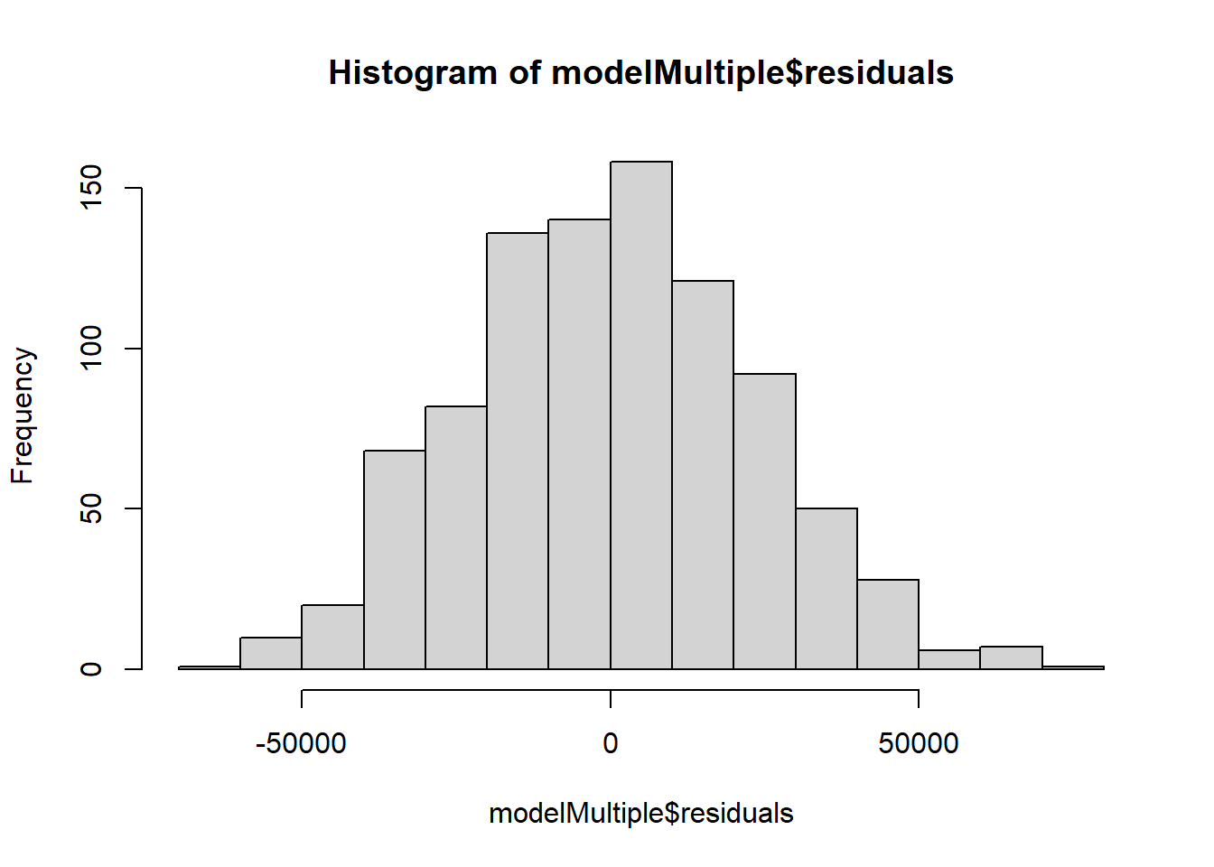
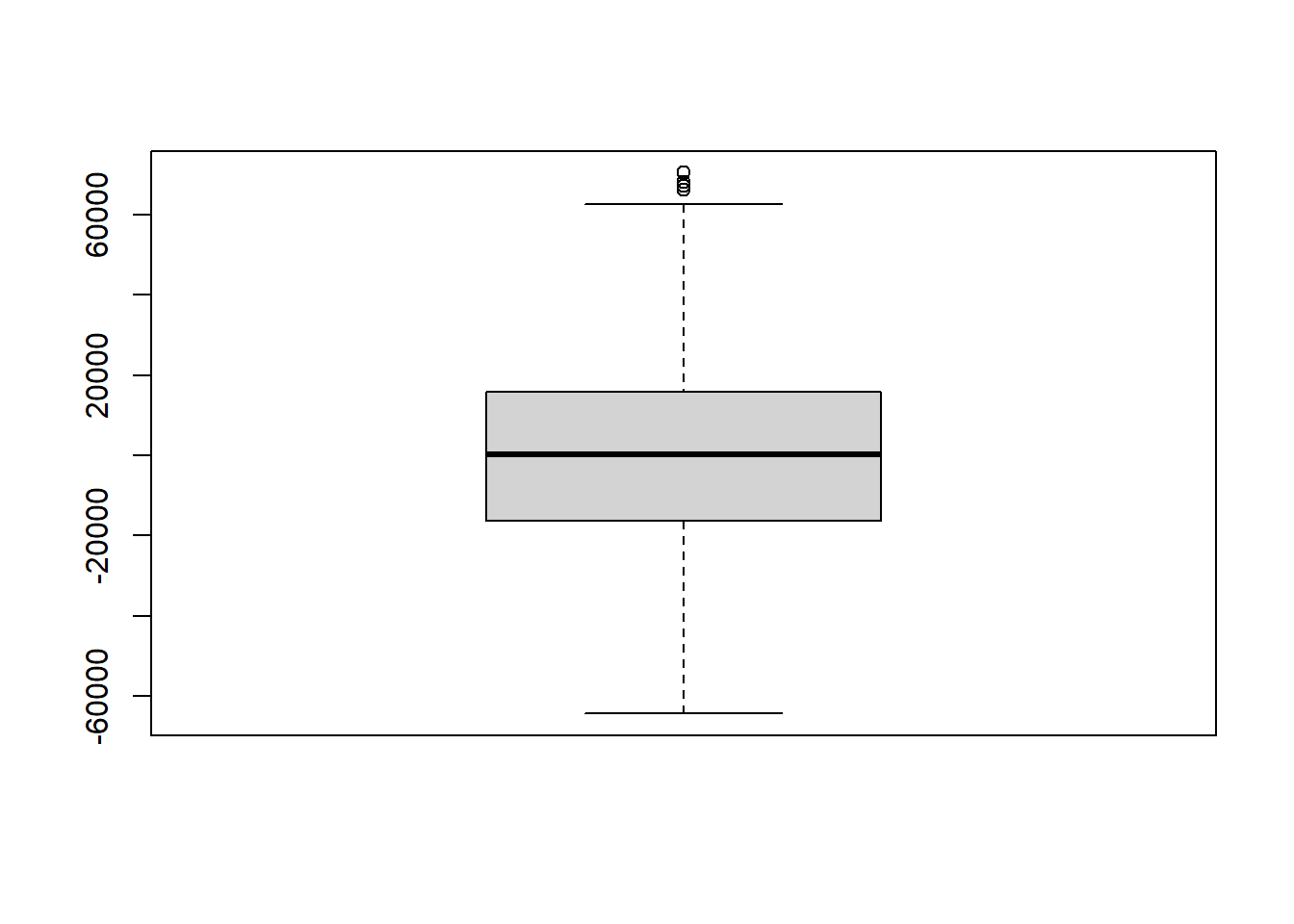
To test the normality assumption of our multiple linear regression model, we can look at a histogram and boxplot of the model’s residuals:


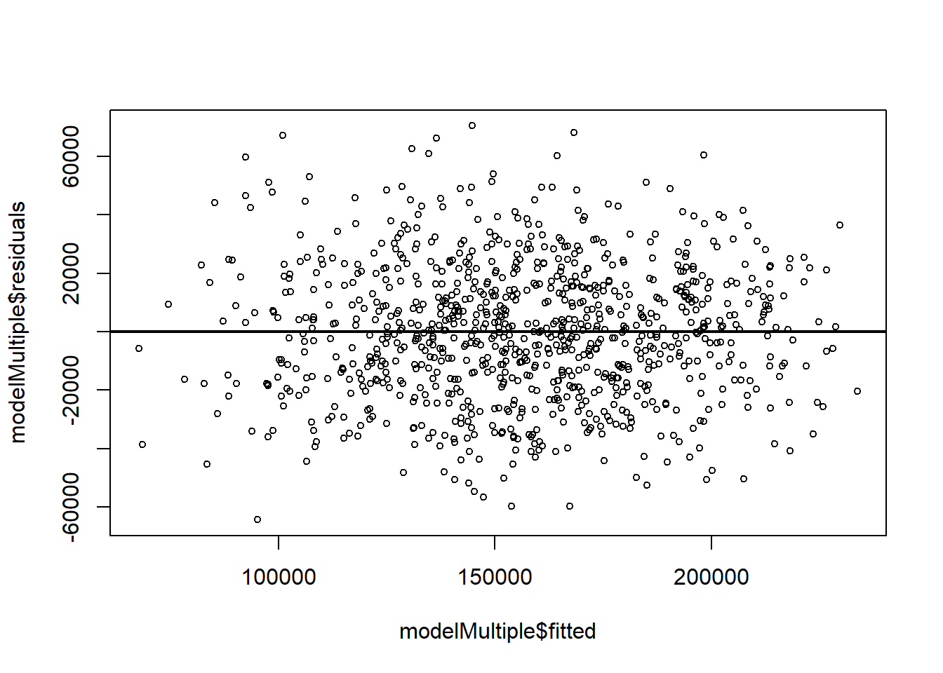
To check for linearity and constant variance, we can create a scatter plot of the residuals v. fitted values of the model:

Because we have nested models (modelSimple is a subset of modelMultiple) we can run an F-test using the anova() command:
## Analysis of Variance Table
##
## Model 1: Salary ~ Age
## Model 2: Salary ~ Age + Rating + Gender + Degree
##   Res.Df        RSS Df  Sum of Sq      F    Pr(>F)
## 1    918 9.7755e+11
## 2    912 4.9163e+11  6 4.8592e+11 150.23 < 2.2e-16 ***
## ---
## Signif. codes:  0 '***' 0.001 '**' 0.01 '*' 0.05 '.' 0.1 ' ' 1
The small p-value suggests that the additional variables in modelMultiple (Rating, Gender, and Degree) do provide predictive ability.
We can use the AIC() function to compare the AIC of the models:
##               df      AIC
## modelSimple    3 21738.07
## modelMultiple  9 21117.74
5.4 Prediction
To apply our models to new observations, we can use the predict() function. Suppose we want to predict the salary of a female employee who is 50, has a rating of eight, and has a Master’s degree.
The predict() function allows us to apply our models to this new data set.
##        1
## 168475.1## 1
## 182445.7