Chapter 7 Machine Learning (DDM)

7.1 Model Building

7.1.1 Elastic net

Elastic net logistic regression allows us to fit a logistic regression model with L1 and L2 regularization parameters, balanced by the hyperparameter \(\alpha\) (alpha). To tune the regularization parameter \(\lambda\) we can use \(k\)-fold cross validation.

We can implement this in R with the cv.glmnet() function from the glmnet package. Unlike other modeling functions we have seen, this function requires the feature variables (\(X\)s) to be stored in a matrix and the outcome variable (\(Y\)) to be stored in a factor vector.

x <- Matrix(as.matrix(churn[,c("account_length", "total_day_minutes", "total_day_calls")]), sparse = TRUE)
y <- as.factor(churn$churn)
modelGlmnet <- cv.glmnet(x, y, alpha = 0.8, family = 'binomial', 
                         type.measure = "class", nlambda = 100)

7.1.2 Random forest

We can fit a random forest model in R with the ranger() function from the ranger package. The syntax for this function is more similar to the lm() and glm() function we saw in previous sections:

modelRF <- ranger(churn ~ ., data = churn, 
                  probability = TRUE, importance = "impurity")

7.2 Model Evaluation

In this section, we will evaluate our modelRF model on a holdout set called test. First, we use the predict() function to apply our model to the test set and store the result into rfPreds. We can access the model’s prediction for each observation in test by accessing $predictions within rfPreds.

rfPreds <- predict(modelRF, test)
head(rfPreds$predictions)

##           [,1]        [,2]
## [1,] 0.2915074 0.708492600
## [2,] 0.9557985 0.044201503
## [3,] 0.9098254 0.090174603
## [4,] 0.9924437 0.007556349
## [5,] 0.9584230 0.041576964
## [6,] 0.9252328 0.074767157

The second column above contains the predicted probability that the observation equals 1. To calculate a confusion matrix for our model, we pass the predictions along with the realizations into the confusionMatrix() function from the caret package.

To convert our model’s predicted probabilities to a discrete prediction, we count the model’s prediction as 1 if the probability is greater than 0.5 and 0 otherwise (which is stored in preds below). Note that for the confusionMatrix function, both the predictions and realizations need to be stored as factors.

preds <- as.factor(as.numeric(rfPreds$predictions[,2] > 0.5))
reals <- as.factor(test$churn)

confusionMatrix(preds, reals)

## Confusion Matrix and Statistics
## 
##           Reference
## Prediction   0   1
##          0 906  49
##          1  19  89
##                                         
##                Accuracy : 0.936         
##                  95% CI : (0.9196, 0.95)
##     No Information Rate : 0.8702        
##     P-Value [Acc > NIR] : 2.177e-12     
##                                         
##                   Kappa : 0.688         
##                                         
##  Mcnemar's Test P-Value : 0.0004368     
##                                         
##             Sensitivity : 0.9795        
##             Specificity : 0.6449        
##          Pos Pred Value : 0.9487        
##          Neg Pred Value : 0.8241        
##              Prevalence : 0.8702        
##          Detection Rate : 0.8523        
##    Detection Prevalence : 0.8984        
##       Balanced Accuracy : 0.8122        
##                                         
##        'Positive' Class : 0             
## 

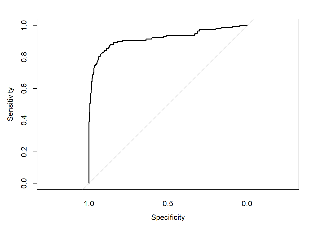
We can calculate the AUC of our model and plot the ROC curve with the roc() and auc() functions from the pROC package:

rocObj <- roc(test$churn, rfPreds$predictions[,2])

auc(rocObj)

## Area under the curve: 0.9166

plot(rocObj)