3 Classification Models
Both regression and classification are types of supervised learning in machine learning, where a model learns from labeled data to make predictions on unseen data. The key difference lies in the nature of the target variable: regression predicts continuous values, while classification predicts categorical classes.
At the Table 3.1 summarizes their main distinctions:
| Aspect | Regression | Classification |
|---|---|---|
| Objective | Predict continuous numerical values | Predict categorical class labels |
| Output Variable (\(y\)) | Continuous (real numbers) | Discrete (finite set of categories) |
| Model Form | \(f(x) \rightarrow y\) | \(f(x) \rightarrow C_i\) |
| Examples of \(y\) | Price, temperature, weight, sales | Spam/Not spam, disease/no disease |
| Error Metric | Mean Squared Error (MSE), MAE, RMSE | Accuracy, Precision, Recall, F1-score |
| Decision Boundary | Not applicable (predicts magnitude) | Separates classes in feature space |
| Probabilistic Output | Direct prediction of numeric value | Often models \(P(y = C_i \mid x)\) |
| Example Algorithms | Linear Regression, Polynomial Regression, Support Vector Regression (SVR) | Logistic Regression, Decision Tree, Random Forest, SVM, Neural Networks |
| Visualization | Regression line or curve | Decision regions or confusion matrix |
3.1 Intro to Classification
Classification is a supervised learning technique used to predict categorical outcomes — that is, assigning data into predefined classes or labels. Mathematically, classification algorithms learn a function:
\[ f(x) \rightarrow y \]
where:
- \(x = [x_1, x_2, \dots, x_n]\): vector of input features (predictors)
- \(y \in \{C_1, C_2, \dots, C_k\}\): categorical class label
- \(f(x)\): the classification function or model that maps inputs to one of the predefined classes
In practice, the classifier estimates the probability that an observation belongs to each class:
\[ P(y = C_i \mid x), \quad i = 1, 2, \dots, k \]
and assigns the class with the highest probability:
\[ \hat{y} = \arg\max_{C_i} P(y = C_i \mid x) \]
Thus, classification involves learning a decision boundary that separates different classes in the feature space.
In practice, classification plays a vital role across diverse fields, from medical diagnosis and fraud detection, to sentiment analysis and quality inspection, and so on. Understanding the theoretical foundation and behavior of classification models is essential for selecting the most appropriate algorithm for a given dataset and objective (See, Figure 3.1).
3.2 Decision Tree
A Decision Tree is a non-linear supervised learning algorithm used for both classification and regression tasks. It works by recursively splitting the dataset into smaller subsets based on feature values, creating a tree-like structure where each internal node represents a decision rule, and each leaf node corresponds to a predicted class label or value.
Decision Trees are intuitive, easy to interpret, and capable of capturing non-linear relationships between features and the target variable.
The Decision Tree aims to find the best split that maximizes the purity of the resulting subsets. The quality of a split is measured using impurity metrics such as:
Gini Index \[ Gini = 1 - \sum_{i=1}^{k} p_i^2 \]
Entropy (Information Gain) \[ Entropy = - \sum_{i=1}^{k} p_i \log_2(p_i) \]
Information Gain \[ IG(D, A) = Entropy(D) - \sum_{v \in Values(A)} \frac{|D_v|}{|D|} Entropy(D_v) \]
where:
- \(p_i\) = proportion of samples belonging to class i
- \(D\) = dataset before split
- \(A\) = attribute used for splitting
- \(D_v\) = subset of \(D\) for which attribute \(A\) has value \(v\)
The algorithm selects the feature and threshold that maximize Information Gain (or minimize Gini impurity).
3.2.1 CART Algorithm
The CART (Classification and Regression Tree) algorithm builds binary trees by recursively splitting data into two subsets based on a threshold value. It uses:
- Gini impurity for classification tasks, and
- Mean Squared Error (MSE) for regression tasks.
For a feature \(X_j\) and threshold \(t\), CART finds the split that minimizes:
\[ Gini_{split} = \frac{N_L}{N} Gini(L) + \frac{N_R}{N} Gini(R) \]
where:
- \(N_L\), \(N_R\) = number of samples in left and right nodes
- \(L\), \(R\) = left and right subsets after split
- \(N\) = total samples before split
- Produces binary splits only
- Supports both classification and regression
- Basis for Random Forests and Gradient Boosted Trees
3.2.2 ID3 Algorithm
The Iterative Dichotomiser 3 (ID3 algorithm) builds a decision tree using Information Gain as the splitting criterion. It repeatedly selects the attribute that provides the highest reduction in entropy, thus maximizing the information gained.
At each step:
\[ InformationGain(D, A) = Entropy(D) - \sum_{v \in Values(A)} \frac{|D_v|}{|D|} Entropy(D_v) \]
- Uses Entropy and Information Gain
- Works well with categorical features
- Can overfit if not pruned
- Forms the foundation for C4.5
3.2.3 C4.5 Algorithm
The C4.5 algorithm is an improvement over ID3, addressing its limitations by:
- Handling continuous and categorical data
- Managing missing values
- Using Gain Ratio instead of pure Information Gain
- Supporting tree pruning to prevent overfitting
The Gain Ratio is defined as:
\[ GainRatio(A) = \frac{InformationGain(D, A)}{SplitInformation(A)} \]
where:
\[ SplitInformation(A) = -\sum_{v \in Values(A)} \frac{|D_v|}{|D|} \log_2\left(\frac{|D_v|}{|D|}\right) \]
- More robust than ID3
- Can handle continuous attributes (by setting threshold splits)
- Reduces bias toward attributes with many distinct values
- Forms the basis for modern tree algorithms like C5.0
3.2.4 Comparison Decision Tree
The following table (see, Table 3.2) compares the most popular Decision Tree algorithms — ID3, C4.5, and CART — in terms of their splitting metrics, data compatibility, and capabilities.
| Algorithm | Splitting Metric | Data Type | Supports Continuous? | Handles Missing Values? | Pruning |
|---|---|---|---|---|---|
| ID3 | Information Gain | Categorical | ❌ | ❌ | ❌ |
| C4.5 | Gain Ratio | Mixed | ✅ | ✅ | ✅ |
| CART | Gini / MSE | Mixed | ✅ | ✅ | ✅ |
3.3 Probabilistic Models
Probabilistic models are classification models based on the principles of probability theory and Bayesian inference. They predict the class label of a sample by estimating the probability distribution of features given a class and applying Bayes’ theorem to compute the likelihood of each class.
A probabilistic classifier predicts the class \(y\) for an input vector \(x = (x_1, x_2,\cdots, x_n)\) as:
\[ \hat{y} = \arg\max_y \; P(y|x) \]
Using Bayes’ theorem:
\[ P(y|x) = \frac{P(x|y) P(y)}{P(x)} \]
Since \(P(x)\) is constant across all classes:
\[ \hat{y} = \arg\max_y \; P(x|y) P(y) \]
3.3.1 Naive Bayes
Naive Bayes is a simple yet powerful probabilistic classifier based on Bayes’ theorem, with the naive assumption that all features are conditionally independent given the class label.
General formula for Naive Bayes model:
\[ P(y|x_1, x_2, ..., x_n) \propto P(y) \prod_{i=1}^{n} P(x_i|y) \]
where:
- \(P(y)\) = prior probability of class \(y\)
- \(P(x_i|y)\) = likelihood of feature \(x_i\) given class \(y\)
The predicted class is:
\[ \hat{y} = \arg\max_y \; P(y) \prod_{i=1}^{n} P(x_i|y) \]
- Gaussian Naive Bayes → assumes continuous features follow a normal distribution
- Multinomial Naive Bayes → for discrete counts (e.g., word frequencies in text)
- Bernoulli Naive Bayes → for binary features (e.g., spam detection)
3.3.2 LDA
Linear Discriminant Analysis (LDA) is a probabilistic classifier that assumes each class follows a multivariate normal (Gaussian) distribution with a shared covariance matrix but different means. It projects the data into a lower-dimensional space to maximize class separability. General formula for LDA model,
For class \(k\):
\[ P(x|y=k) = \frac{1}{(2\pi)^{d/2} |\Sigma|^{1/2}} \exp\left(-\frac{1}{2}(x - \mu_k)^T \Sigma^{-1} (x - \mu_k)\right) \]
Decision rule:
\[ \hat{y} = \arg\max_k \; \delta_k(x) \]
where:
\[ \delta_k(x) = x^T \Sigma^{-1} \mu_k - \frac{1}{2} \mu_k^T \Sigma^{-1} \mu_k + \log P(y=k) \]
- Assumes equal covariance matrices across classes
- Decision boundaries are linear
- Works well for normally distributed features
3.3.3 QDA
Quadratic Discriminant Analysis (QDA) is an extension of LDA that allows each class to have its own covariance matrix. This flexibility enables non-linear decision boundaries. General formula for QDA model,
For class \(k\):
\[ P(x|y=k) = \frac{1}{(2\pi)^{d/2} |\Sigma_k|^{1/2}} \exp\left(-\frac{1}{2}(x - \mu_k)^T \Sigma_k^{-1} (x - \mu_k)\right) \]
Decision function:
\[ \delta_k(x) = -\frac{1}{2} \log|\Sigma_k| - \frac{1}{2}(x - \mu_k)^T \Sigma_k^{-1} (x - \mu_k) + \log P(y=k) \]
- Allows different covariance matrices → more flexible
- Decision boundaries are quadratic (nonlinear)
- Requires more data than LDA to estimate covariance matrices
3.3.4 Logistic Regression
Logistic Regression is a probabilistic linear model used for binary classification. It estimates the probability that an input belongs to a particular class using the logistic (sigmoid) function. General formula for Logistic Regression model:
Let \(x\) be the input vector and \(\beta\) the coefficient vector:
\[ P(y=1|x) = \frac{1}{1 + e^{-(\beta_0 + \beta^T x)}} \]
Decision rule:
\[ \hat{y} = \begin{cases} 1, & \text{if } P(y=1|x) \ge 0.5 \\ 0, & \text{otherwise} \end{cases} \]
The model is trained by maximizing the likelihood function (or equivalently, minimizing the negative log-likelihood):
\[ L(\beta) = \sum_{i=1}^{n} [y_i \log P(y_i|x_i) + (1 - y_i)\log(1 - P(y_i|x_i))] \]
- Produces linear decision boundaries
- Interpretable model coefficients
- Can be extended to multiclass classification using Softmax Regression
3.3.5 Comparison Probabilistics
The following table (Table 3.3) compares four popular probabilistic models — Naive Bayes, LDA, QDA, and Logistic Regression — based on their underlying assumptions, mathematical structure, and flexibility.
| Model | Assumptions | Decision Boundary | Covariance | Handles Continuous? | Nonlinear? |
|---|---|---|---|---|---|
| Naive Bayes | Feature independence | Linear (in log-space) | N/A | ✅ | ❌ |
| LDA | Gaussian, shared covariance | Linear | Shared (Σ) | ✅ | ❌ |
| QDA | Gaussian, class-specific covariance | Quadratic | Separate (Σₖ) | ✅ | ✅ |
| Logistic Regression | Linear log-odds | Linear | Implicit | ✅ | ❌ |
3.4 Kernel Methods
Kernel methods are a family of machine learning algorithms that rely on measuring similarity between data points rather than working directly in the original feature space. They are especially useful for non-linear classification, where data are not linearly separable in their original form. By using a kernel function, these methods implicitly project data into a higher-dimensional feature space, allowing linear separation in that transformed space — without explicitly performing the transformation.
3.4.1 SVM
Support Vector Machine (SVM) is a powerful supervised learning algorithm that seeks to find the optimal hyperplane that separates classes with the maximum margin. It can handle both linear and non-linear classification problems. For a binary classification problem, given data points \((x_i, y_i)\) where \(y_i \in \{-1, +1\}\):
The objective is to find the hyperplane:
\[ w^T x + b = 0 \]
such that the margin between the two classes is maximized:
\[ \min_{w, b} \frac{1}{2} \|w\|^2 \]
subject to:
\[ y_i (w^T x_i + b) \ge 1, \quad \forall i \]
In the nonlinear case, SVM uses a kernel function \(K(x_i, x_j)\) to implicitly map data into a higher-dimensional space:
\[ K(x_i, x_j) = \phi(x_i)^T \phi(x_j) \]
| Kernel | Formula | Description |
|---|---|---|
| Linear | \(K(x_i, x_j) = x_i^T x_j\) | Simple linear separation |
| Polynomial | \(K(x_i, x_j) = (x_i^T x_j + c)^d\) | Captures polynomial relations |
| RBF (Gaussian) | \(K(x_i, x_j) = \exp(-\gamma \|x_i - x_j\|^2)\) | Nonlinear, smooth decision boundary |
| Sigmoid | \(K(x_i, x_j) = \tanh(\alpha x_i^T x_j + c)\) | Similar to neural networks |
Characteristics Kernel Functions in SVM (see, Table 3.4):
- Maximizes margin between classes (robust to outliers)
- Works in high-dimensional spaces
- Supports nonlinear separation using kernels
- Sensitive to kernel choice and hyperparameters (e.g., \(C\), \(\gamma\))
3.4.2 KNN
K-Nearest Neighbors (KNN) is a non-parametric, instance-based learning algorithm. It classifies a new data point based on the majority class of its k closest training samples, according to a chosen distance metric. For a new observation \(x\), compute its distance to all training samples \((x_i, y_i)\):
\[ d(x, x_i) = \sqrt{\sum_{j=1}^{n} (x_j - x_{ij})^2} \]
Then, select the k nearest neighbors and assign the class by majority voting:
\[ \hat{y} = \arg\max_c \sum_{i \in N_k(x)} I(y_i = c) \]
where:
- \(N_k(x)\) = indices of the k nearest points
- \(I(y_i = c)\) = indicator function (1 if true, 0 otherwise)
| Metric | Formula | Typical Use |
|---|---|---|
| Euclidean Distance | \(d(x, y) = \sqrt{\sum_i (x_i - y_i)^2}\) | Continuous / numerical features |
| Manhattan Distance | \(d(x, y) = \sum_i |x_i - y_i|\) | Sparse or grid-like data |
| Minkowski Distance | \(d(x, y) = (\sum_i |x_i - y_i|^p)^{1/p}\) | Generalized form (includes Euclidean & Manhattan) |
| Cosine Similarity | \(\text{sim}(x, y) = \frac{x \cdot y}{\|x\| \|y\|}\) | Text data or directional similarity |
| Hamming Distance | \(d(x, y) = \sum_i [x_i \neq y_i]\) | Binary or categorical data |
| Jaccard Similarity | \(J(A, B) = \frac{|A \cap B|}{|A \cup B|}\) | Set-based or binary features |
Characteristics in Distance and Similarity Metrics (see, Table 3.5)
- Lazy learning: no explicit training phase
- Sensitive to feature scaling and noise
- Works best for small to medium datasets
- Decision boundaries can be nonlinear and flexible
3.4.3 Comparison Kernels
The following Table 3.6 presents a comparison of two widely used non-probabilistic classification models: Support Vector Machine (SVM) and K-Nearest Neighbors (KNN). It highlights their key characteristics, including model type, parametric nature, ability to handle nonlinearity, computational cost, interpretability, and important hyperparameters.
| Model | Type | Parametric? | Handles Nonlinearity | Training Cost | Interpretation | Key Hyperparameters |
|---|---|---|---|---|---|---|
| Support Vector Machine (SVM) | Kernel-based | ✅ Yes | ✅ Yes (via kernel) | Moderate to High | Moderate | C, kernel, γ |
| K-Nearest Neighbors (KNN) | Instance-based | ❌ No | ✅ Yes (implicitly) | Low (training) / High (prediction) | High | k, distance metric |
3.5 Ensemble Methods
Ensemble methods are machine learning techniques that combine multiple base models to produce a single, stronger predictive model. The idea is that aggregating diverse models reduces variance, bias, and overfitting, leading to better generalization. Ensemble methods can be categorized into:
- Bagging: Reduces variance by training models on bootstrapped subsets (e.g., Random Forest)
- Boosting: Reduces bias by sequentially training models that focus on previous errors (e.g., Gradient Boosting, XGBoost)
3.5.1 Random Forest
Random Forest is a bagging-based ensemble of Decision Trees. Each tree is trained on a random subset of data with random feature selection, and the final prediction is obtained by majority voting (classification) or averaging (regression). General Form for Random Forest:
- Generate B bootstrap samples from the training data.
- Train a Decision Tree on each sample:
- At each split, consider a random subset of features (m out of p)
- At each split, consider a random subset of features (m out of p)
- Combine predictions:
- Classification:
\[ \hat{y} = \text{mode}\{T_1(x), T_2(x), ..., T_B(x)\} \]
- Regression:
\[ \hat{y} = \frac{1}{B} \sum_{b=1}^{B} T_b(x) \]
- Classification:
- Reduces overfitting compared to single trees
- Works well with high-dimensional and noisy datasets
- Less interpretable than a single tree
3.5.2 Gradient Boosting Machines
GBM is a boosting-based ensemble that builds models sequentially, where each new model tries to correct errors of the previous one. It focuses on minimizing a differentiable loss function (e.g., log-loss for classification). General Form for Gradient Boosting Machines:
Initialize the model with a constant prediction:
\[ F_0(x) = \arg\min_\gamma \sum_{i=1}^n L(y_i, \gamma) \]For \(m = 1\) to \(M\) (number of trees):
- Compute the residuals (pseudo-residuals):
\[ r_{im} = -\left[ \frac{\partial L(y_i, F(x_i))}{\partial F(x_i)} \right]_{F(x) = F_{m-1}(x)} \]
- Fit a regression tree to the residuals
- Update the model:
\[ F_m(x) = F_{m-1}(x) + \nu T_m(x) \]
where \(\nu\) is the learning rate
- Compute the residuals (pseudo-residuals):
- Reduces bias by sequential learning
- Can overfit if too many trees or high depth
- Sensitive to hyperparameters (learning rate, tree depth, number of trees)
3.5.3 Extreme Gradient Boosting
XGBoost is an optimized implementation of Gradient Boosting that is faster and more regularized. It incorporates techniques such as shrinkage, column subsampling, tree pruning, and parallel computation for improved performance. Similar to GBM, but adds regularization to the objective function:
\[ Obj = \sum_{i=1}^{n} L(y_i, \hat{y}_i) + \sum_{k=1}^{K} \Omega(f_k) \]
where:
\[ \Omega(f) = \gamma T + \frac{1}{2} \lambda \sum_{j=1}^{T} w_j^2 \]
- \(T\) = number of leaves in tree \(f\)
- \(w_j\) = leaf weight
- \(\gamma, \lambda\) = regularization parameters
- Fast and scalable
- Handles missing values automatically
- Prevents overfitting with regularization and early stopping
- Widely used in Kaggle competitions
3.5.4 Comparison Ensemble
The following table (see Table 3.7) summarizes key ensemble methods, highlighting their type, main strengths, weaknesses, and the scenarios where they are most effective:
| Method | Type | Strength | Weakness | Best Use Case |
|---|---|---|---|---|
| Random Forest | Bagging | Reduces variance, robust | Less interpretable | High-dimensional, noisy data |
| GBM | Boosting | Reduces bias, accurate | Sensitive to overfitting | Medium datasets, complex patterns |
| XGBoost | Boosting (optimized) | Fast, regularized, accurate | Hyperparameter tuning required | Large datasets, competitive ML tasks |
3.6 Study Case Examples
The following table (see, Table 3.8) summarizes representative applications of classification models across different fields:
| Domain | Application | Description / Objective |
|---|---|---|
| Healthcare | Disease diagnosis | Classify patients as disease vs no disease. |
| Medical imaging | Identify tumor presence in X-ray or MRI scans. | |
| Patient readmission prediction | Use hospital data to forecast readmission risk. | |
| Finance | Credit scoring | Predict whether a customer will default on a loan. |
| Fraud detection | Identify fraudulent credit card transactions. | |
| Investment risk classification | Categorize assets as low, medium, or high risk. | |
| Marketing | Customer churn prediction | Determine whether a customer will leave a service. |
| Target marketing | Segment customers into high vs. low purchase potential. | |
| Lead scoring | Prioritize sales prospects based on conversion likelihood. | |
| Text Mining | Sentiment analysis | Classify text as positive, negative, or neutral. |
| Spam detection | Detect unwanted or harmful emails/messages. | |
| Topic classification | Categorize documents by subject matter. | |
| Transportation | Traffic sign recognition | Classify sign types in autonomous vehicles. |
| Driver behavior analysis | Detect aggressive or distracted driving patterns. | |
| Route classification | Predict optimal routes based on historical data. |
3.7 End to End Study Case
This project demonstrates an end-to-end binary logistic regression analysis using the built-in mtcars dataset in R. We aim to predict whether a car has a Manual or Automatic transmission based on:
mpg— Miles per gallon (fuel efficiency)
hp— Horsepower (engine power)
wt— Vehicle weight
3.7.1 Data Preparation
data("mtcars")
mtcars$am <- factor(mtcars$am, labels = c("Automatic", "Manual"))

str(mtcars)
'data.frame': 32 obs. of 11 variables:
$ mpg : num 21 21 22.8 21.4 18.7 18.1 14.3 24.4 22.8 19.2 ...
$ cyl : num 6 6 4 6 8 6 8 4 4 6 ...
$ disp: num 160 160 108 258 360 ...
$ hp : num 110 110 93 110 175 105 245 62 95 123 ...
$ drat: num 3.9 3.9 3.85 3.08 3.15 2.76 3.21 3.69 3.92 3.92 ...
$ wt : num 2.62 2.88 2.32 3.21 3.44 ...
$ qsec: num 16.5 17 18.6 19.4 17 ...
$ vs : num 0 0 1 1 0 1 0 1 1 1 ...
$ am : Factor w/ 2 levels "Automatic","Manual": 2 2 2 1 1 1 1 1 1 1 ...
$ gear: num 4 4 4 3 3 3 3 4 4 4 ...
$ carb: num 4 4 1 1 2 1 4 2 2 4 ...head(mtcars) mpg cyl disp hp drat wt qsec vs am gear carb
Mazda RX4 21.0 6 160 110 3.90 2.620 16.46 0 Manual 4 4
Mazda RX4 Wag 21.0 6 160 110 3.90 2.875 17.02 0 Manual 4 4
Datsun 710 22.8 4 108 93 3.85 2.320 18.61 1 Manual 4 1
Hornet 4 Drive 21.4 6 258 110 3.08 3.215 19.44 1 Automatic 3 1
Hornet Sportabout 18.7 8 360 175 3.15 3.440 17.02 0 Automatic 3 2
Valiant 18.1 6 225 105 2.76 3.460 20.22 1 Automatic 3 13.7.2 Logistic Regression Model
Let say, you build a model using all variables in the mtcars dataset to predict whether a car has a manual or automatic transmission.
# Load dataset
data("mtcars")
mtcars$am <- factor(mtcars$am, labels = c("Automatic", "Manual"))

# Full logistic regression model using all predictors
full_model <- glm(am ~ ., data = mtcars, family = binomial)

summary(full_model)
Call:
glm(formula = am ~ ., family = binomial, data = mtcars)

Coefficients:
              Estimate Std. Error z value Pr(>|z|)
(Intercept) -1.164e+01  1.840e+06       0        1
mpg         -8.809e-01  2.884e+04       0        1
cyl          2.527e+00  1.236e+05       0        1
disp        -4.155e-01  2.570e+03       0        1
hp           3.437e-01  2.195e+03       0        1
drat         2.320e+01  2.159e+05       0        1
wt           7.436e+00  3.107e+05       0        1
qsec        -7.577e+00  5.510e+04       0        1
vs          -4.701e+01  2.405e+05       0        1
gear         4.286e+01  2.719e+05       0        1
carb        -2.157e+01  1.076e+05       0        1

(Dispersion parameter for binomial family taken to be 1)

    Null deviance: 4.3230e+01  on 31  degrees of freedom
Residual deviance: 6.4819e-10  on 21  degrees of freedom
AIC: 22

Number of Fisher Scoring iterations: 25
Check for Multicollinearity with VIF (Variance Inflation Factor)
# Install if not installed
# install.packages("car")
library(car)

# Calculate VIF values
vif_values <- vif(full_model)

# Sort from highest to lowest
vif_values <- sort(vif_values, decreasing = TRUE)

# Print the results
vif_values
disp cyl wt hp carb mpg gear vs
45.336024 38.112972 28.384837 21.288933 21.096231 18.150446 16.289577 11.102033
qsec drat
9.214178 3.950868 Interpretation of VIF values:
- VIF = 1 → No multicollinearity.
- VIF between 1–5 → Moderate correlation (acceptable).
- VIF > 10 → Serious multicollinearity problem.
Now, compare with the simpler model using only three predictors (mpg, hp, and wt):
model2 <- glm(am ~mpg+wt,
              data = mtcars, family = binomial)

summary(model2)
Call:
glm(formula = am ~ mpg + wt, family = binomial, data = mtcars)

Coefficients:
            Estimate Std. Error z value Pr(>|z|)
(Intercept)  25.8866    12.1935   2.123   0.0338 *
mpg          -0.3242     0.2395  -1.354   0.1759
wt           -6.4162     2.5466  -2.519   0.0118 *
---
Signif. codes:  0 '***' 0.001 '**' 0.01 '*' 0.05 '.' 0.1 ' ' 1

(Dispersion parameter for binomial family taken to be 1)

    Null deviance: 43.230  on 31  degrees of freedom
Residual deviance: 17.184  on 29  degrees of freedom
AIC: 23.184

Number of Fisher Scoring iterations: 7vif(model2) mpg wt
3.556491 3.556491 # Dataset
data(mtcars)
mtcars$am <- factor(mtcars$am, labels = c("Automatic", "Manual"))
# Untuk analisis korelasi, ubah am ke numerik (0/1)
mtcars$am_num <- as.numeric(mtcars$am) - 1library(ggcorrplot)
# Hitung matriks korelasi
cor_mat <- cor(mtcars[, sapply(mtcars, is.numeric)])
# Plot
ggcorrplot(cor_mat,
hc.order = TRUE,
type = "lower",
lab = TRUE,
lab_size = 3,
colors = c("red", "white", "blue"),
title = "Heatmap Korelasi Variabel Numerik - mtcars",
ggtheme = ggplot2::theme_minimal())
library(ggplot2)
cor_vals <- cor(mtcars[, sapply(mtcars, is.numeric)])
am_corr <- sort(cor_vals["am_num", -which(colnames(cor_vals) == "am_num")])

# Ubah ke data frame untuk ggplot
df_corr <- data.frame(Variable = names(am_corr),
                      Correlation = am_corr)

ggplot(df_corr, aes(x = reorder(Variable, Correlation), y = Correlation, fill = Correlation)) +
  geom_col() +
  coord_flip() +
  scale_fill_gradient2(low = "red", high = "blue", mid = "white", midpoint = 0) +
  labs(title = "Korelasi Variabel terhadap Transmisi (am)",
       x = NULL, y = "Koefisien Korelasi") +
  theme_minimal()
The model estimates the probability that a car is Manual using the formula:
\[ \log\left(\frac{p}{1-p}\right) = \beta_0 + \beta_1(\text{mpg}) + \beta_2(\text{hp}) + \beta_3(\text{wt}) \]
3.7.3 Prediction and Classification
mtcars$prob <- predict(model2, type = "response")

mtcars$pred_class <- ifelse(mtcars$prob > 0.5, "Manual", "Automatic")

head(mtcars[, c("mpg", "wt", "am", "prob", "pred_class")])
mpg wt am prob pred_class
Mazda RX4 21.0 2.620 Manual 0.90625492 Manual
Mazda RX4 Wag 21.0 2.875 Manual 0.65308276 Manual
Datsun 710 22.8 2.320 Manual 0.97366320 Manual
Hornet 4 Drive 21.4 3.215 Automatic 0.15728804 Automatic
Hornet Sportabout 18.7 3.440 Automatic 0.09561351 Automatic
Valiant 18.1 3.460 Automatic 0.10149089 Automatic3.7.4 Confusion Matrix
conf_mat <- table(Actual = mtcars$am, Predicted = mtcars$pred_class)
conf_mat
Predicted
Actual Automatic Manual
Automatic 18 1
Manual 1 12Interpretation:
- Diagonal values show correct predictions
- Off-diagonal values show misclassifications
The following plot illustrates how well the model separates the two classes based on predicted probabilities.
library(ggplot2)
library(dplyr)

conf_data <- table(Actual = mtcars$am, Predicted = mtcars$pred_class) %>%
  as.data.frame()

ggplot(conf_data, aes(x = Predicted, y = Actual, fill = Freq)) +
  geom_tile(color = "white") +
  geom_text(aes(label = Freq), size = 6, color = "black") +
  scale_fill_gradient(low = "white", high = "steelblue") +
  labs(
    title = "Confusion Matrix Heatmap",
    x = "Predicted Class",
    y = "Actual Class",
    fill = "Count"
  ) +
  theme_minimal(base_size = 14)
3.7.5 Evaluation Metrics
TP <- conf_mat["Manual", "Manual"]
TN <- conf_mat["Automatic", "Automatic"]
FP <- conf_mat["Automatic", "Manual"]
FN <- conf_mat["Manual", "Automatic"]

Accuracy  <- (TP + TN) / sum(conf_mat)
Precision <- TP / (TP + FP)
Recall    <- TP / (TP + FN)
F1_Score  <- 2 * (Precision * Recall) / (Precision + Recall)

metrics <- data.frame(
  Metric = c("Accuracy", "Precision", "Recall", "F1 Score"),
  Value  = round(c(Accuracy, Precision, Recall, F1_Score), 3)
)
metrics
Metric Value
1 Accuracy 0.938
2 Precision 0.923
3 Recall 0.923
4 F1 Score 0.923| Metric | Description |
|---|---|
| Accuracy | Overall correctness of predictions |
| Precision | How precise the “Manual” predictions are |
| Recall | Ability to detect all Manual cars |
| F1 Score | Harmonic mean of Precision and Recall |
3.7.6 ROC Curve and AUC
library(pROC)Type 'citation("pROC")' for a citation.
Attaching package: 'pROC'The following objects are masked from 'package:stats':
cov, smooth, varroc_obj <- roc(mtcars$am, mtcars$prob)Setting levels: control = Automatic, case = ManualSetting direction: controls < casesauc_value <- auc(roc_obj)
plot(roc_obj, col = "#2C7BB6", lwd = 2, main = "ROC Curve for Logistic Regression")
abline(a = 0, b = 1, lty = 2, col = "gray")
text(0.6, 0.2, paste("AUC =", round(auc_value, 3)), col = "black")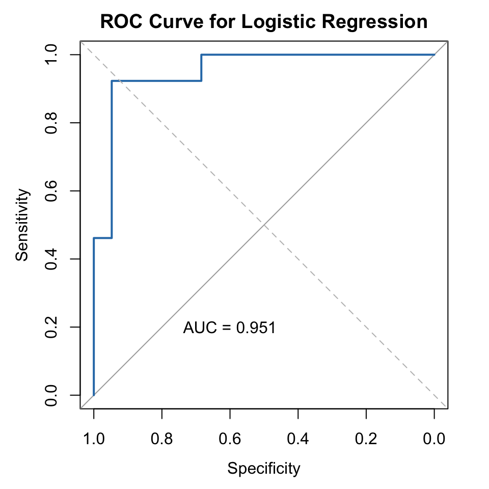
Interpretation:
- The ROC curve shows the trade-off between True Positive Rate and False Positive Rate
- AUC (Area Under the Curve) evaluates how well the model distinguishes between classes
- AUC = 1 → Perfect
- AUC ≥ 0.8 → Excellent
- AUC = 0.5 → Random guessing
- AUC = 1 → Perfect
3.7.7 Conclusion
The logistic regression model successfully predicts car transmission type (Manual vs Automatic) with strong performance.
| Aspect | Result / Interpretation |
|---|---|
| Significant variable | wt (vehicle weight) has a negative effect on Manual probability |
| Model accuracy | ≈ 90% |
| AUC | > 0.8 (Excellent discriminative power) |
| Conclusion | The model performs well in classifying car transmissions |