Chapter 4 Expectation and Variance

4.1 Expectation (Mean)

Given a list of numbers $x_1, x_2,\ldots, x_n$, the familiar way to average them is to add them up and divide by $n$. This is called the arithmetic mean, and is defined by \[ \bar{x}=\frac{1}{n}\sum_{j=1}^{n} x_j. \] More generally, we can define a weighted mean of $x_1,\ldots,x_n$ as

\[ \mbox{weighted-mean}(x)=\sum_{j=1}^{n} x_j p_j, \] where the weights $p_1,\ldots,p_n$ are pre-specified nonnegative numbers that add up to 1 (so the unweighted mean is obtained when $p_j = 1/n$ for all $j$).

Definition 4.1.1 (Expectation of a discrete r.v.).

The expected value (also called the expectation or mean) of a discrete r.v. $X$ whose distinct possible values are $x_1,x_2,\ldots$ is defined by \[ E(X)=\sum_{j=1}^{\infty} x_j P(X=x_j). \]

If the support is finite, then this is replaced by a finite sum.

We can also write \[ E(X)=\sum_x x P(X=x), \] where the sum is over the support of $X$ (in any case, $xP(X = x)$ is 0 for any $x$ not in the support).

The mean may not exist for a probability distribution!

The expectation is undefined if $\sum_{j=1}^{\infty} |x_j| P(X=x_j)$ diverges, since then the series for $E(X)$ diverges or its value depends on the order in which the $x_j$ are listed (conditionally convergent series).

Examples:

Let $X$ be the result of rolling a fair 6-sided die, so $X$ takes on the values 1, 2, 3, 4, 5, 6, with equal probabilities. Intuitively, we should be able to get the average by adding up these values and dividing by 6. Using the definition, the expected value is

\[ E(X)=\frac{1}{6}(1+2+\ldots+6)=3.5. \]

Let $X\sim\mbox{Bern}(p)$ and $q=1-p$. Then

\[ E(X)=1p+0q=p. \]

Let $X\sim Bin(4, 1/2)$, then its PMF can be written by (tabular form)

x	0	1	2	3	4
$p_X(x)$	1/16	4/16	6/16	4/16	1/16

\[ E(X)=0*1/16+1*4/16+2*6/16+3*4/16+4*1/16=2=np \]

The interpretation would be to consider a large number of independent Bernoulli trials, each with probability $p$ of success. Writing 1 for “success” and 0 for “failure”, in the long run we would expect to have data consisting of $np$ successes.

Proposition 4.1.2.

If $X$ and $Y$ are discrete r.v.s with the same distribution, then $E(X) = E(Y)$ (if either side exists).

The converse of the above proposition is false since the expected value is just a one-number summary, not nearly enough to specify the entire distribution; it’s a measure of where the “center” is but does not determine, for example, how spread out the distribution is or how likely the r.v. is to be positive.

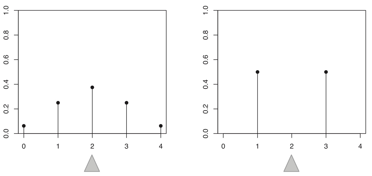
Figure 4.1: Two different distributions with identical mean:

4.2 Expectation of functions of r.v.

For example, given r.v. $X$, a function of r.v. is \[ Y=g(X) \] which is also a r.v.

We can also a function of two different r.v.s, such as $Z=X+Y$.

How to obtain the expectation for a function of r.v.?

Can we simply use \[ E(Y)=g(E(X))? \] It depends on the function!

4.3 Properties of expectation - Linearity and Monotonicity

Theorem 4.2.1 (Linearity of expectation).

For any r.v.s $X$, $Y$ and any constant $c$, \[ E(X+Y) = E(X)+E(Y) \]

\[ E(cX) = cE(X). \]

The expectation of a linear combination of r.vs is the the linear combination of their expectations. Regardless of independence between $X$ and $Y$!

Example 4.2.2 (Binomial expectation).

For $X\sim\mbox{Bin}(n, p)$, let’s find $E(X)$ in two ways.

Recall: Bernoulli and Binomial relationship

Binomial r.v. is made of $n$ independent Bernoulli r.v.s \[ X=X_1+\cdots+X_n \] where $X_j \sim Bernoulli(p), \quad j=1,\ldots, n$. \[ E(X)=E(X_1+\cdots+X_n)=E(X_1)+\cdots+E(X_n)=p+\ldots+p=np \]

Example 4.2.3 (Hypergeometric expectation).

Let $X\sim\mbox{HGeom}(w,b,n)$, interpreted as the number of white balls in a sample of size $n$ drawn without replacement from an urn with $w$ white and $b$ black balls. As in the Binomial case, we can write $X$ as a sum of Bernoulli random variables, \[ X= I_1+\ldots I_n, \] where $I_j$ equals 1 if the $j$th ball in the sample is white and 0 otherwise.

$I_j\sim\mbox{Bern}(p)$ with $p=w/(w+b)$, since unconditionally the $j$th ball drawn is equally likely to be any of the balls.
Unlike in the Binomial case, the $I_j$ are not independent, since the sampling is without replacement: given that a ball in the sample is white, there is a lower chance that another ball in the sample is white. However, linearity still holds for dependent random variables! Thus,

\[ E(X)=n\frac{w}{w+b}. \]

Proposition 4.2.4 (Monotonicity of expectation).

Let $X$ and $Y$ be r.v.s such that $X\geq Y$ with probability 1. Then $E(X) \geq E(Y)$, with equality holding if and only if $X=Y$ with probability 1.

Proof.

This result holds for all r.v.s, but we will prove it only for discrete r.v.s since this chapter focuses on discrete r.vs. The r.v. $Z=X-Y$ is nonnegative (with probability 1), so $E(Z)\geq 0$, since $E(Z)$ is defined as a sum of nonnegative terms. By linearity, \[ E(X)-E(Y)=E(X-Y) \geq 0, \] as desired.

If $E(X)=E(Y)$, then by linearity we also have $E(Z)=0$, which implies that $P(X = Y) = P(Z = 0) = 1$ since if even one term in the sum defining $E(Z)$ is positive, then the whole sum is positive.

4.4 Geometric distribution

Story 4.3.1 (Geometric distribution).

Consider a sequence of independent Bernoulli trials, each with the same success probability $p\in (0, 1)$, with trials performed until a success occurs. Let $X$ be the number of failures before the first successful trial. Then $X$ has the Geometric distribution with parameter $p$; we denote this by $X\sim\mbox{Geom}(p)$.
For example, if we flip a fair coin until it lands Heads for the first time, then the number of Tails before the first occurrence of Heads is distributed as $\mbox{Geom}(1/2)$.

To get the Geometric PMF from the story, imagine the Bernoulli trials as a string of 0’s (failures) ending in a single 1 (success). Each 0 has probability $q=1-p$ and the final 1 has probability $p$, so a string of $k$ failures followed by one success has probability $q^k p$.

Theorem 4.3.2 (Geometric PMF).

If $X\sim\mbox{Geom}(p)$, then the PMF of $X$ is \[ P (X=k)=q^k p \] for $k=0,1,2,\ldots$, where $q=1-p$.

This is a valid PMF because

\[ \sum_{k=0}^\infty q^k p=p\sum_{k=0}^\infty q^k=p\cdot \frac{1}{(1-q)}=1. \]

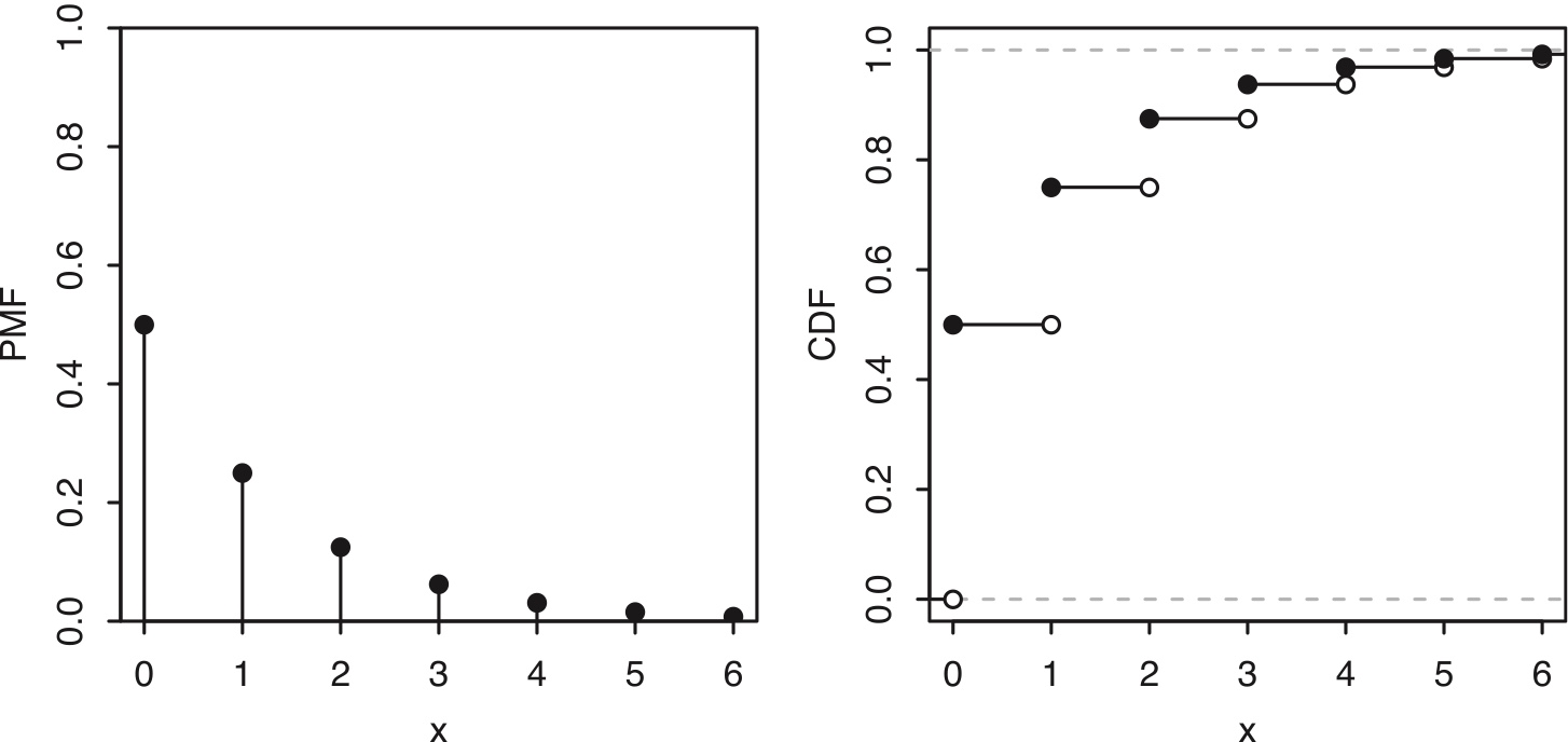
Figure 4.2: PMF and CDF of a geometric distribution

There are differing conventions for the definition of the Geometric distribution; some sources define the Geometric as the total number of trials, including the success. In this book, the Geometric distribution excludes the success.

Example 4.3.5 (Geometric expectation).

\[ P (X=k)=q^k p,\quad k=0,1,2,\ldots \]

\[ E(X)=\sum_{k=0}^\infty kq^kp=0+qp+2q^2p+3q^3p+\cdots=p(0+q+2q^2+3q^3+\cdots) \]

The one in the parenthesis is no long the sum of a geometric series.

However, the term $kq^k$ looks like the form of derivative respect to $q^k$.

We know that \[ \frac{1}{1-q}=\sum_{k=0}^\infty q^k. \] If we take derivative on both sides, we have \[ \frac{1}{(1-q)^2}=\sum_{k=0}^\infty kq^{k-1}=\frac{\sum_{k=0}^\infty kq^{k}}{q}. \]

Finally we have \[ E(X)=\sum_{k=0}^\infty kq^kp=0+qp+2q^2p+3q^3p+\cdots=p(0+q+2q^2+3q^3+\cdots)=p\cdot \frac{q}{(1-q)^2}=\frac{q}{p} \] Recall: Odds of success \[ \text{odds}=\frac{p}{q} \]

4.5 Memoryless Property of Geometric Distribution

Let $X$ be a random variable that follows a Geometric distribution with success probability $p$:

\[ P(X = k) = q^{k} p, \quad k = 0, 1, 2, 3, \dots \]

Then $X$ has the memoryless property, which means

\[ P(X > m + n \mid X > m) = P(X > n) \]

for all nonnegative integers $m, n$.

If $X$ represents the number of failures until the first success, then the probability that you will need to go through more than $n$ additional failures , given that you’ve already went through $m$ failures without success, is the same as if you were starting over.

Poof (hint: using the CDF of Geometric distribution)

4.6 Negative Binomial distribution

Story 4.3.7 (Negative Binomial distribution).

In a sequence of independent Bernoulli trials with success probability $p$, if $X$ is the number of failures before the $r$th success, then $X$ is said to have the Negative Binomial distribution with parameters $r$ and $p$, denoted $X\sim\mbox{NBin}(r, p)$.

Both the Binomial and the Negative Binomial distributions are based on independent Bernoulli trials; they differ in the stopping rule and in what they are counting: the Binomial counts the number of successes in a fixed number of trials, while the Negative Binomial counts the number of failures until a fixed number of successes.

Theorem 4.3.8 (Negative Binomial PMF).

If $X\sim\mbox{NBin(r,p)}$, then the PMF of $X$ is \[ P(X=n)={n+r-1\choose r-1}p^r q^n \] for $n=0,1,2,\ldots$, where $q=1-p$.

Theorem 4.3.9.

Let $X\sim \mbox{NBin}(r, p)$, viewed as the number of failures before the rth success in a sequence of independent Bernoulli trials with success probability $p$. Then we can write $X = X_1+\ldots +X_r$ where the $X_i$ are i.i.d. $\mbox{Geom}(p)$.

$X_1$ is the number of failures before the 1st success
$X_2$ is the number of failures between the 1st and 2nd success
… …
$X_r$ is the number of failures between the $(r-1)$th success and the $r$th success

Example 4.3.10 (Negative Binomial expectation).

\[ r\cdot\frac{q}{p} \]

4.7 Expectation of a nonlinear function of an r.v.

If we have a function of random variable $X$, such as $Y=g(X)$, if $g$ is linear function, we already know the expectation of $Y$ is \[ E(Y)=g(E(X)) \] However, if $g$ is not linear, we do not have $E(Y)=g(E(X))$ in general!

Example 4.3.14 (St. Petersburg paradox).

Suppose a wealthy stranger offers to play the following game with you. You will flip a fair coin until it lands Heads for the first time, and you will receive $2 if the game lasts for 1 round, $4 if the game lasts for 2 rounds, $8 if the game lasts for 3 rounds, and in general, $$2^n$ if the game lasts for $n$ rounds.

What is the expectation of the reward?

(Use the alternative parameterization of Geometric distribution)

In the generic definition of Geometric distribution, the r.v. is the number of failures that we go through before the 1st success.

Geometric distribution has an alternative formulation. We can also define the r.v. $X$ as the number of trials we have to try to obtain 1st success. \[ P(X=n)=q^{n-1}p=(1/2)^n,\quad n=1,2,\ldots \] The value of reward is a function of $X$, which is $2^X$. Denote the value of reward as $Y$, then $Y=2^X$.

What is the expectation of $Y$? Is it simply $2^{E(X)}$?

Anyway, let’s find $E(X)$ first.

From the generic parameterization of Geometric distribution, we know the expectation of failures until the first success is $q/p=1$. Of course the expectation of the trials (including failure and the last success) is $2$.

Can we say $E(Y)=2^2=4$?

We can validate it using the definition of method to find the expectation of $Y$. \[ \begin{split} P(Y=2)&=P(X=1)=(1/2) \\ P(Y=4)&=P(X=2)=(1/2)^2=\frac{1}{4} \\ P(Y=8)&=P(X=3)=(1/2)^3=\frac{1}{8} \\ \dots \end{split} \]

By the definition of expectation, \[ E(Y)=2*\frac{1}{2}+4*\frac{1}{4}+\cdots=1+1+\cdots=\infty \]

4.8 Law of the unconscious statistician (LOTUS)

For a general function $g(x)$, which is not necessarily linear, the expectation of $g(X)$ can be obtained by so-called Law of the unconscious statistician (LOTUS).

Theorem 4.5.1 (LOTUS).

If $X$ is a discrete r.v. and $g$ is a function from $\mathbb{R}$ to $\mathbb{R}$, then \[ E(g(X))=\sum_x g(x) P(X=x), \] where the sum is taken over all possible values of $X$.

If we have PMF of r.v. $X$:

X	$x_1$	$x_2$	…
$p_X$	$P(X=x_1)$	$P(X=x_2)$	…

Then the PMF of $Y=g(X)$ will be \[ P(Y=y)=P(X=x)=p_X(x) \]

Y=g(X)	$g(x_1)$	$g(x_2)$	…
$p_Y$	$P(X=x_1)$	$P(X=x_2)$	…

Of course, the expectation of $Y$ is \[ E(Y)=E(g(X))=\sum_x g(x) P(X=x). \]

4.9 Indicator r.v.s and the fundamental bridge

An indicator r.v. $I_A$ (or $I(A)$) for an event $A$ is defined to be 1 if $A$ occurs and 0 otherwise, \[ I_A = \left\{ \begin{array}{rl} 1 & \mbox{if A occurs} \\ 0 & \mbox{if A does not occur.} \end{array}\right. \]

The Bernoulli random r.v, is a typical indicator r.v, which indicates the occurrence of “success”.

Theorem 4.4.1 (Properties of Indicator r.v.)

Let $A$ and $B$ be events. Then the following properties hold.

$(I_A)^k=I_A$ for any positive integer $k$.
$I_{A^c}=1-I_A$.
$I_{A\cap B}=I_A I_B$.
$I_{A\cup B}=I_A+I_B-I_A I_B$.

Theorem 4.4.2 (Fundamental bridge between probability and expectation).

The expectation of the indicator r.v. $I_A$ is the probability of the event $A$, \[ E(I_A)=P(A). \]

For example, the expectation of Bernoulli($p$) is $p$.

Example 4.4.3 (Boole, Bonferroni, and inclusion-exclusion).

Let $A_1,A_2,\ldots,A_n$ be events. Note that \[ I(A_1\cup\ldots\cup A_n)\leq I(A_1)+\ldots +I(A_n). \] Taking the expectation of both sides and using linearity and the fundamental bridge, we have \[ P(A_1\cup\ldots\cup A_n)\leq P(A_1)+\ldots +P(A_n), \] which is called Boole’s inequality or Bonferroni’s inequality.

Proof of Inclusion-exclusion theorem:

To prove inclusion-exclusion for $n=2$, we can take the expectation of both sides in Property 4 of Theorem 4.4.1.

For general $n$, we can use properties of indicator r.v.s as follows: \[ \begin{split} 1-I(A_1\cup\ldots \cup A_n) & = I(A_1^c\cap\ldots\cap A_n^c) \\ \\ & = (1-I(A_1))\ldots (1-I(A_n)) \\ \\ & = 1-\sum_i I(A_i)+\sum_{i<j} I(A_i)I(A_j)-\ldots \\ \\ & + (-1)^n I(A_1)\ldots I(A_n). \end{split} \] Taking the expectation of both sides, by the fundamental bridge we have inclusion-exclusion.

We are trying to find $P(A_1\cup \cdots\cup A_n)$.

By de Morgan’s Law, \[ (A_1\cup \cdots\cup A_n)^c=A_1^c\cap \cdots\cap A_n^c \] Thus \[ I((A_1\cup \cdots\cup A_n)^c)=I(A_1^c\cap \cdots\cap A_n^c) \]

\[ 1-I(A_1\cup \cdots\cup A_n)=I(A_1^c\cap \cdots\cap A_n^c)=(1-I(A_1))\cdots((1-I(A_n)) \]

Example 4.4.4 (Matching continued).

We have a well-shuffled deck of $n$ cards, labeled 1 through $n$. A card is a match if the card’s position in the deck matches the card’s label.

Define $I_j$ as the indicator r.v., which indicates the $j$th card is a match, so \[ X=I_1+\cdots+I_n. \] and \[ E(X)=E(I_1)+E(I_2)+\cdots+E(I_n) \] Now, let’s find $E(I_j)$.

Since $I_j$ is an indicator r.v., \[ E(I_j)=P(I_j=1)=\frac{(n-1)!}{n!}=\frac{1}{n} \] Thus, \[ E(X)=nE(I_j)=1 \]

Example 4.4.5 (Distinct birthdays, birthday matches).

In a group of $n$ people, under the usual assumptions about birthdays, what is the expected number of distinct birthdays among the $n$ people, i.e., the expected number of days on which at least one of the people was born? (Use the property of indicator r.v.)

Define indicator r.v. $I_j$, which indicates at least one person was born on that day, $j=1,2,\ldots, 365$.

Define r.v. $X$ as the number of days one which at least one person was born, then \[ X=I_1+\cdots+I_{365}. \] We have \[ E(X)=E(I_1)+\cdots+E(I_{365}). \]

Now, lets find $E(I_j)$. \[ E(I_j)=P(I_j=1)=1-\frac{364^n}{365^n} \] Thus, \[ E(X)=n(1-\frac{364^n}{365^n}) \]

Example 4.4.6 (Putnam problem).

A permutation $a_1,a_2,\ldots,a_n$ of $1,2,\ldots,n$ has a local maximum at $j$ if $a_j>a_{j-1}$ and $a_j>a_{j+1}$ (for $2\leq j\leq n-1$; for $j=1$, a local maximum at $j$ means $a_1>a_2$ while for $j=n$ it means $a_n>a_{n-1}$).

For example, 4, 2, 5, 3, 6, 1 has 3 local maxima, at positions 1, 3, and 5.

The Putnam exam from 2006 posed the following question: for $n\geq 2$, what is the average number of local maxima of a random permutation of $1, 2,\ldots,n$, with all $n!$ permutations equally likely?

Define indicator r.v. $I_j$, which indicates $j$th number in the permutation is a local maxima.

For $j=1$ or $j=n$, \[ P(I_j=1)=\frac{1}{2} \] For $j=2, \ldots, n-1$, \[ P(I_j=1)=\frac{2}{3!}=\frac{1}{3} \] Define $X$ as the total number of local maxima, \[ X=I_1+I_2+\cdots+I_{n-1}+I_n. \]

\[ E(X)=E(I_1)+E(I_2)+\cdots+E(I_{n-1})+E(I_n)=2*1/2+(n-2)*1/3. \]

4.10 Negative Hypergeometric

Example 4.4.7 (Negative Hypergeometric).

An urn contains $w$ white balls and $b$ black balls, which are randomly drawn one by one without replacement, until $r$ white balls have been obtained ($r<w$).

The number of black balls drawn before drawing the $r$th white ball has a Negative Hypergeometric distribution with parameters $w$, $b$, $r$. We denote this distribution by $\mbox{NHGeom}(w,b,r)$.

For example, if we shuffle a deck of cards and deal them one at a time, the number of cards dealt before uncovering the first ace is $\mbox{NHGeom}(4,48,1)$.

As another example, suppose a college offers $g$ good courses and $b$ bad courses (for some definition of “good” and “bad”), and a student wants to find 4 good courses to take. Not having any idea which of the courses are good, the student randomly tries out courses one at a time, stopping when they have obtained 4 good courses. Then the number of bad courses the student tries out is $\mbox{NHGeom}(g,b,4)$.

We can obtain the PMF of $X\sim \mbox{NHGeom}(w,b,r)$ by imagining that we continue drawing balls until the urn has been emptied out; this is valid since whether or not we continue to draw balls after obtaining the $r$th white ball has no effect on $X$.

Think of the $w+b$ balls as lined up in a random order, the order in which they will be drawn.

Then $X=k$ means that among the first $r+k-1$ balls there are exactly $r-1$ white balls, then there is a white ball, and then among the last $w+b-r-k$ balls there are exactly $w-r$ white balls.
All ${w+b\choose w}$ possibilities for the locations of the white balls in the line are equally likely. So by the naive definition of probability, we have the following expression for the PMF:

\[ P(X=k)=\frac{{r+k-1\choose r-1}{w+b-r-k\choose w-r}}{{w+b\choose w}},\;\;k=0,\ldots,b. \]

Finding the expected value of a Negative Hypergeometric r.v. directly from the definition of expectation results in complicated sums. But the answer is very simple: for $X\sim\mbox{NHGeom}(w,b,r)$, we have $E(X)=rb/(w+1)$.

Sanity check : This answer makes sense since it is increasing in $b$, decreasing in $w$, and correct in the extreme cases $b = 0$ (when no black balls will be drawn) and $w = 0$ (when all the black balls will be exhausted before drawing a nonexistent white ball).

Closely related to indicator r.v.s is an alternative expression for the expectation of a nonnegative integer-valued r.v. $X$. Rather than summing up values of $X$ times values of the PMF of $X$, we can sum up probabilities of the form $P(X > n)$ (known as tail probabilities), over nonnegative integers $n$.

The following table shows the distributions for four sampling schemes: the sampling can be done with or without replacement, and the stopping rule can require a fixed number of draws or a fixed number of successes.

	With replacement	Without replacement
Fixed number of trials	Binomial	Hypergeometric
Fixed number of successes	Negative Binomial	Negative Hypergeometric

4.11 Variance

One important application of LOTUS is for finding the variance of a random variable. Like expected value, variance is a single-number summary of the distribution of a random variable. While the expected value tells us the center of mass of a distribution, the variance tells us how spread out the distribution is.

Definition 4.6.1 (Variance and standard deviation).

The variance of an r.v. $X$ is \[ Var(X)=E[X-E(X)]^2. \] The square root of the variance is called the standard deviation (SD): \[ SD(X)=\sqrt{Var(X)}. \]

Theorem 4.6.2. (Alternative formula to calculate variance)

For any r.v. $X$, \[ Var(X)=E(X^2)-[E(X)]^2. \]

Properties of Variance:

$Var(X+c)=Var(X)$ for any constant $c$.
$Var(cX)=c^2Var(X)$ for any constant $c$.
$Var(cX+b)=c^2Var(X)$ for any constant $c$ and $b$.
If $X$ and $Y$ are independent, then $Var(X+Y)=Var(X)+Var(Y)$. This is not true in general if $X$ and $Y$ are dependent.
$Var(X)\geq 0$, with equality if and only if $P(X=a)=1$ for some constant $a$. In other words, the only random variables that have zero variance are constants (which can be thought of as degenerate r.v.s); all other r.v.s have positive variance.

4.6.3 (Variance is not linear).

Unlike expectation, variance is not linear. The constant comes out squared in $Var(cX)=c^2Var(X)$, and the variance of the sum of r.v.s may or may not be the sum of their variances.

Example 4.6.4-part1 Variance of Geometric distribution.

For geometric distribution $Geom(p)$ \[ P(X=x)=q^x p, \quad x=0, 1, 2,\ldots \]

Use the alternative formula to calculate $Var(X)$: \[ Var(X)=E(X^2)-[E(X)]^2 \]

We already have $E(X)=q/p$. \[ E(X^2)=\sum_{x=0}^\infty x^2q^xp=p\sum_{x=0}^\infty x^2q^x \] To find the $\sum_{x=0}^\infty x^2q^x$, we use the same tricks we used to find $E(X)$.

Take derivative of \[ \sum_{x=0}^\infty q^x=\frac{1}{1-q}, \] respect to $q$ for twice. \[ \sum_{x=0}^\infty xq^{x-1}=\frac{1}{(1-q)^2} \]

\[ \sum_{x=0}^\infty xq^{x}=\frac{q}{(1-q)^2}=\frac{q}{1+q^2-2q} \]

\[ \sum_{x=0}^\infty x^2q^{x-1}=\frac{1+q^2-2q-q(2q-2)}{(1-q)^4}=\frac{1+q}{(1-q)^3} \]

\[ \sum_{x=0}^\infty x^2q^{x}=\frac{1+q^2-2q-q(2q-2)}{(1-q)^4}=\frac{q(1+q)}{(1-q)^3} \]

Thus, \[ E(X^2)=\frac{pq(1+q)}{(1-q)^3}=\frac{q(1+q)}{p^2} \] For $Geom(p)$, its variance is \[ Var(X)=E(X^2)-[E(X)]^2=\frac{q(1+q)}{p^2}-\left(\frac{q}{p}\right)^2=\frac{q}{p^2} \]

Example 4.6.4-part2 Variance of Negative binomial distribution.

If $X\sim\mbox{NBin(r,p)}$, then $X$ can be represented as
\[ X = X_1+\ldots +X_r \] where the $X_i$ are i.i.d. $\mbox{Geom}(p)$.

For independent variables $X_1,\ldots,X_r$, the total variance is additive, \[ Var(X)=Var(X_1)+\cdots+Var(X_r)=r\cdot\frac{q}{p} \]

Example 4.6.5 (Binomial variance).

If $X\sim Bin(n, p)$, then $X$ can be represented as \[ X=X_1+X_2+\cdots+X_n, \] where $X_i\overset{iid}{\sim} Bernoulli(p)$.

Again, used additivity of variance for independent r.v.s, \[ Var(X)=n\cdot Var(X_i) \]

To find the variance of Bernoulli r.v., we can use the alternative formula of variance, \[ Var(X_i)=E(X_i^2)-[E(X_i)]^2=E(X_i^2)-p^2 \]

After taking a square, $X_i^2$ is still a Bernoulli variable with the exact same distribution, which is $Bernoulli(p)$. Thus, \[ E(X_i^2)=p. \]

\[ Var(X_i)=p-p^2=p(1-p)=pq \]

Finally, we have \[ Var(X)=npq \]

4.12 Poisson

Definition 4.7.1 (Poisson distribution).

An r.v. $X$ has the Poisson distribution with parameter $\lambda$ if the PMF of $X$ is \[ P(X=k)=\frac{e^{-\lambda}\lambda^k}{k!},\;\; k=0,1,2,\ldots \] We write this as $X\sim\mbox{Pois}(\lambda)$.

Example 4.7.2 (Poisson expectation and variance).

004x007-eps-converted-to

The Poisson distribution is often used in situations where we are counting the number of successes in a particular region or interval of time, and there are a large number of trials, each with a small probability of success. For example, the following random variables could follow a distribution that is approximately Poisson.

The number of emails you receive in an hour. There are a lot of people who could potentially email you in that hour, but it is unlikely that any specific person will actually email you in that hour. Alternatively, imagine subdividing the hour into milliseconds. There are $3.6\times 10^6$ seconds in an hour, but in any specific millisecond it is unlikely that you will get an email.
The number of chips in a chocolate chip cookie. Imagine subdividing the cookie into small cubes; the probability of getting a chocolate chip in a single cube is small, but the number of cubes is large.
The number of earthquakes in a year in some region of the world. At any given time and location, the probability of an earthquake is small, but there are a large number of possible times and locations for earthquakes to occur over the course of the year.

The parameter $\lambda$ is interpreted as the rate of occurrence of these rare events; in the examples above, $\lambda$ could be 20 (emails per hour), 10 (chips per cookie), and 2 (earthquakes per year). The Poisson paradigm says that in applications similar to the ones above, we can approximate the distribution of the number of events that occur by a Poisson distribution.

Approximation 4.7.3 (Poisson paradigm).

Let $A_1,A_2,\ldots, A_n$ be events with $p_j=P(A_j)$, where $n$ is large, the $p_j$ are small, and the $A_j$ are independent or weakly dependent. Let \[ X=\sum_{j=1}^n I(A_j) \] count how many of the $A_j$ occur. Then $X$ is approximately $\mbox{Pois}(\lambda)$ with $\lambda=\sum_{j=1}^n p_j$.

The Poisson paradigm is also called the law of rare events. The interpretation of “rare” is that the $p_j$ are small, not that $\lambda$ is small. For example, in the email example, the low probability of getting an email from a specific person in a particular hour is offset by the large number of people who could send you an email in that hour.

In the examples we gave above, the number of events that occur isn’t exactly Poisson because a Poisson random variable has no upper bound, whereas how many of $A_1,\ldots,A_n$ occur is at most $n$, and there is a limit to how many chocolate chips can be crammed into a cookie. But the Poisson distribution often gives good approximations. Note that the conditions for the Poisson paradigm to hold are fairly flexible: the $n$ trials can have different success probabilities, and the trials don’t have to be independent, though they should not be very dependent. So there are a wide variety of situations that can be cast in terms of the Poisson paradigm. This makes the Poisson a popular model, or at least a starting point, for data whose values are nonnegative integers (called count data in statistics).

Example 4.7.4 (Balls in boxes). There are $k$ distinguishable balls and $n$ distinguishable boxes. The balls are randomly placed in the boxes, with all $n^k$ possibilities equally likely. Problems in this setting are called occupancy problems, and are at the core of many widely used algorithms in computer science.

Find the expected number of empty boxes.

Define $I_j$ as the indicator r.v. for the $j$th box being empty. \[ E(I_j)=P(\text{jth box being empty})=\frac{(n-1)^k}{n^k} \]

\[ E(I_1+\cdots+I_n)=n\left(\frac{n-1}{n}\right)^k \]
Find the probability that at least one box is empty. Express your answer as a sum of at most $n$ terms.

We only discuss the case $k>n$, since when $k<n$, there will always be at least one box empty.

Define $I_j$ as the indicator r.v. for the $j$th box being empty. The event “at least one box is empty” can be written as \[ I_1\cup \cdots \cup I_n \]

\[ \begin{split} P(I_1\cup \cdots \cup I_n)&=\sum_{j=1}^nP(I_j)-\sum_{i<j}P(I_j\cap I_j)+\sum_{i<j<l}P(I_i\cap I_j\cap I_l) \\ &-\cdots+(-1)^nP(I_1\cap \cdots\cap I_n) \end{split} \]

\[ P(I_j)=\frac{(n-1)^k}{n^k} \\ P(I_i\cap I_j)=\frac{(n-2)^k}{n^k} \\ P(I_i\cap I_j\cap I_k)=\frac{(n-3)^k}{n^k} \\ \cdots \]

\[ \begin{split} P(I_1\cup \cdots \cup I_n)&=\binom{n}{1}\frac{(n-1)^k}{n^k}-\binom{n}{2}\frac{(n-2)^k}{n^k}+\binom{n}{3}\frac{(n-3)^k}{n^k} \\ &-\cdots +(-1)^n0 \\ &=\sum_{j=1}^n (-1)^{j-1}\binom{n}{j}\frac{(n-j)^k}{n^k} \end{split} \]
Now let $n=1000$, $k=5806$. The expected number of empty boxes is then approximately 3. Find a good approximation as a decimal for the probability that at least one box is empty. The handy fact $e^3\approx 20$ may help.

The number of empty boxes $X\sim Poisson(\lambda=3)$, \[ P(\text{at least one one box is empty})=P(X\ge 0)=1-P(X=0)=1-\frac{e^{-3}3^0}{0!}\approx 19/20 \]