Chapter 5 Chapter 5: Continuous Distributions

5.1 Probability density function (PDF)

• For a discrete r.v., the CDF jumps at every point in the support, and is flat everywhere else.

• For for a continuous r.v. the CDF increases smoothly;

• See Figure for a comparison of discrete vs. continuous CDFs.

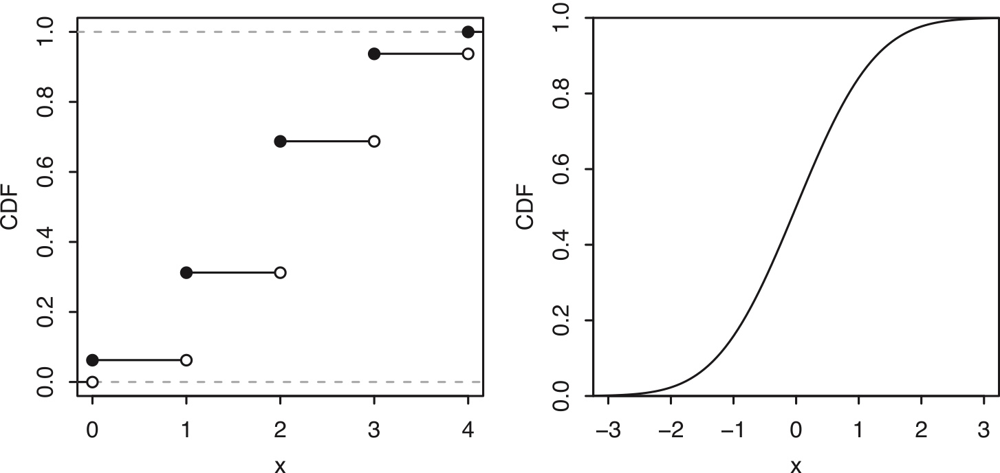
Figure 5.1: Discrete vs. continuous r.v.s. Left: The CDF of a discrete r.v. has jumps at each point in the support. Right: The CDF of a continuous r.v. increases smoothly.

Definition 5.1.1 (Continuous r.v.).

An r.v. has a continuous distribution if its CDF is differentiable. We also allow there to be endpoints (or finitely many points) where the CDF is continuous but not differentiable, as long as the CDF is differentiable everywhere else. A continuous random variable is a random variable with a continuous distribution.

A continuous random variable (r.v.) is a random variable that can take any value within one or more intervals on the real number line.

Definition 5.1.2 (Probability density function (PDF)).

For a continuous r.v. \(X\) with CDF \(F\) , the probability density function (PDF) of \(X\) is the derivative \(f\) of the CDF, given by \(f(x)=F'(x)\). The support of \(X\), and of its distribution, is the set of all \(x\) where \(f(x)>0\).

• An important way in which continuous r.v.s differ from discrete r.v.s is that for a continuous r.v. \(X\), \(P(X=x)=0\) for all \(x\). This is because \(P(X=x)\) is the height of a jump in the CDF at \(x\), but the CDF of \(X\) has no jumps! Since the PMF of a continuous r.v. would just be 0 everywhere, we work with a PDF instead.

• For a PDF \(f\) , the quantity \(f(x)\) is not a probability, and in fact it is possible to have \(f(x)>1\) for some values of \(x\). To obtain a probability, we need to integrate the PDF. The fundamental theorem of calculus tells us how to get from the PDF back to the CDF.

Proposition 5.1.3 (PDF to CDF).

Let \(X\) be a continuous r.v. with PDF \(f\). Then the CDF of \(X\) is given by \[ F(x)=\int_{-\infty}^x f(t) dt. \] Proof. By the definition of PDF, \(F\) is an antiderivative of \(f\). So by the fundamental theorem of calculus, \[ \int_{-\infty}^x f(t) dt=F(x)-F(-\infty)=F(x). \]

• The above result is analogous to how we obtained the value of a discrete CDF at \(x\) by summing the PMF over all values less than or equal to \(x\); here we integrate the PDF over all values up to \(x\), so the CDF is the accumulated area under the PDF.

• Since we can freely convert between the PDF and the CDF using the inverse operations of integration and differentiation, both the PDF and CDF carry complete information about the distribution of a continuous r.v.

• Since the PDF determines the distribution, we should be able to use it to find the probability of \(X\) falling into an interval \((a, b)\). A handy fact is that we can include or exclude the endpoints as we wish without altering the probability, since the endpoints have probability 0:

\[ P(a< X < b)=P(a< X \leq b)=P(a\leq X < b)=P(a\leq X \leq b). \]

Biohazard 5.1.4 (Including or excluding endpoints).

We can be carefree about including or excluding endpoints as above for continuous r.v.s, but we must not be careless about this for discrete r.v.s. By the definition of CDF and the fundamental theorem of calculus, \[ P(a<X\leq b)=F(b)-F(a)=\int_a^b f(x)dx. \] Therefore, to find the probability of \(X\) falling in the interval \((a, b]\) (or \((a, b)\), \([a, b)\), or \([a, b])\) using the PDF, we simply integrate the PDF from \(a\) to \(b\). In general, for an arbitrary region \(A\subseteq \mathbb{R}\), \[ P(X\in A)=\int_A f(x)dx. \]

For continuous distributions, the probability mass distributed on a specific point is negligible!

Theorem 5.1.5 (Valid PDFs).

The PDF \(f\) of a continuous r.v. must satisfy the following two criteria:

• Nonnegative: \(f(x)\geq 0\);
• integrates to \(\int_{-\infty}^{\infty}f(x)dx=1\).

If you have a function \(h(x)\) only satisfy the first condition (nonnegativity), it can be normalized to make it satisfy the second condition by dividing the normalizing constant \[ c=\int_{-\infty}^{\infty}h(x)dx \] This process is called normalization. After that \(f(x)=\frac{h(x)}{c}\) is a valid pdf.

Proof. The first criterion is true because probability is nonnegative; if \(f(x_0)\) were negative, then we could integrate over a tiny region around \(x_0\) and get a negative probability. The second criterion is true since \(\int_{-\infty}^{\infty}f(x)dx\) is the probability of \(X\) falling somewhere on the real line, which is 1.

Conversely, any such function \(f\) is the PDF of some r.v. This is because if \(f\) satisfies these properties, we can integrate it as in Proposition 5.1.3 to get a function \(F\) satisfying the properties of a CDF. Then a version of Universality of the Uniform, the main concept in Section 5.3, can be used to create an r.v. with CDF \(F\).

Example 5.1.6 (Logistic).

The Logistic distribution has CDF \[ F(x)=\frac{e^x}{1+e^x},\;\; x\in\mathbb{R} \] and PDF \[ f(x)=\frac{e^x}{(1+e^x)^2},\;\; x\in\mathbb{R}. \] Let \(X\sim\mbox{Logistic}\). To find \(P(-2<X<2)\), we need to integrate the PDF from -2 to 2.

\[ P(-2<X<2)=F(2)-F(-2) \]

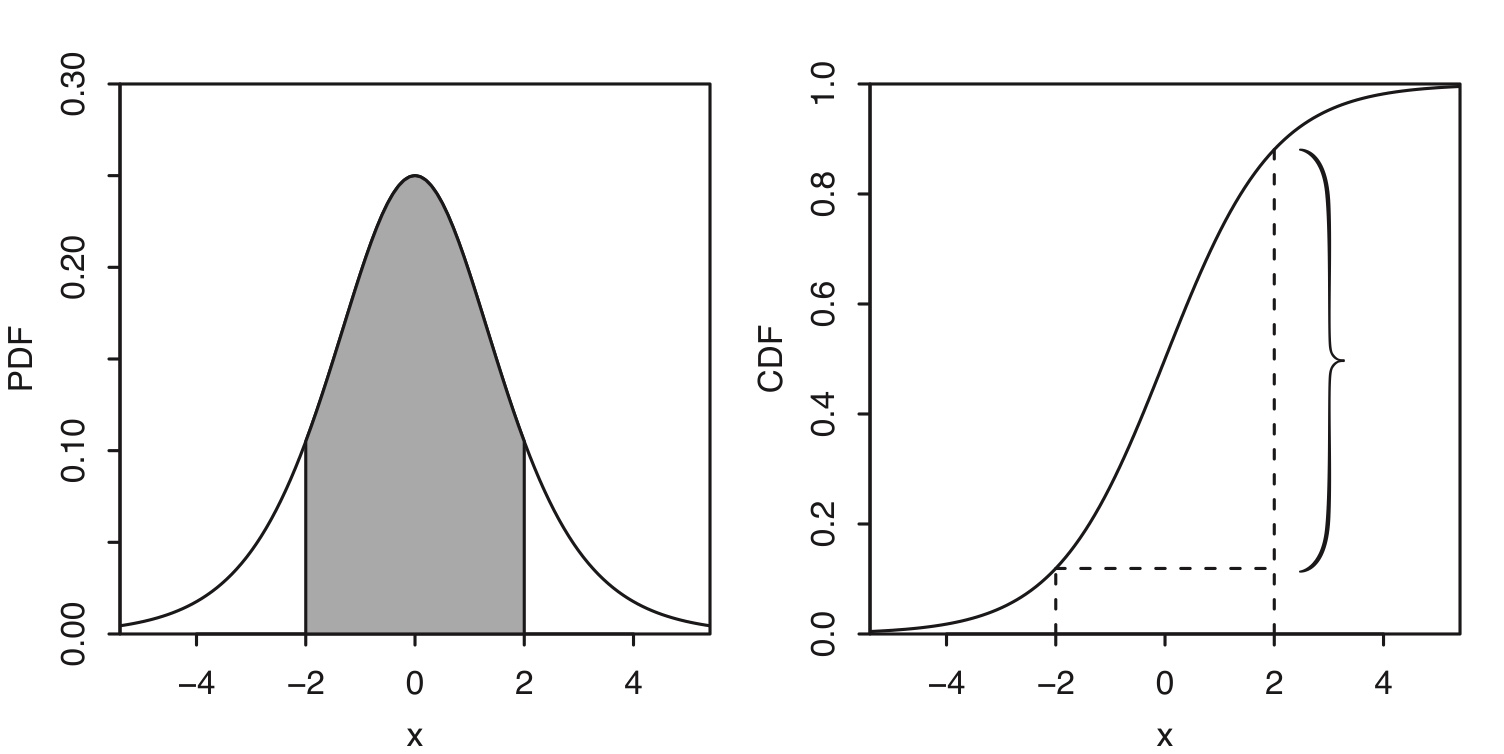
Figure 5.2: Logistic PDF and CDF. The probability \(P(-2<X<2)\) is indicated by the shaded area under the PDF and the height of the curly brace on the CDF.

Example 5.1.7 (Rayleigh).

The Rayleigh distribution has CDF \[ F(x)=1-e^{-x^2/2},\;\; x>0 \] and PDF \[ f(x)=xe^{-x^2/2}\;\; x>0. \] Let \(X\sim\mbox{Rayleigh}\). To find \(P(X>2)\), we need to integrate the PDF from 2 to \(\infty\).

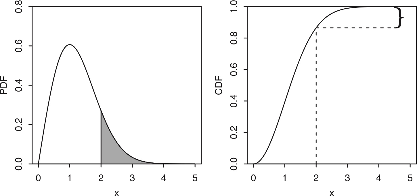
Figure 5.3: Rayleigh PDF and CDF. The probability \(P(X>2)\) is indicated by the shaded area under the PDF and the height of the curly brace on the CDF.

Although the height of a PDF at \(x\) does not represent a probability, it is closely related to the probability of falling into a tiny interval around \(x\), as the following intuition explains.

Intuition 5.1.8.

Let \(F\) be the CDF and \(f\) be the PDF of a continuous r.v. \(X\). As mentioned earlier, \(f(x)\) is not a probability; for example, we could have \(f(3)>1\), and we know \(P(X = 3)=0\). But thinking about the probability of \(X\) being very close to 3 gives us a way to interpret \(f(3)\). Specifically, the probability of \(X\) being in a tiny interval of length \(\epsilon\), centered at 3, will essentially be \(f(3)\epsilon\). This is because \[ P(3-\epsilon/2 < X < 3+\epsilon/2)=\int_{3-\epsilon/2}^{3+\epsilon/2}f(x)dx\approx f(3)\epsilon, \] if the interval is so tiny that \(f\) is approximately the constant \(f(3)\) on that interval. In general, we can think of \(f(x)dx\) as the probability of \(X\) being in an infinitesimally small interval containing \(x\), of length \(dx\).

In practice, \(X\) often has units in some system of measurement, such as units of distance, time, area, or mass. Thinking about the units is not only important in applied problems, but also it often helps in checking that answers make sense. Suppose for concreteness that \(X\) is a length, measured in centimeters (cm). Then \(f(x)=dF(x)/dx\) is the probability per cm at x, which explains why \(f(x)\) is a probability density. Probability is a dimensionless quantity (a number without physical units), so the units of \(f(x)\) are \(\mbox{cm}^{-1}\). Therefore, to be able to get a probability again, we need to multiply \(f(x)\) by a length. When we do an integral such as \(\int_0^5 f(x)dx\) , this is achieved by the often-forgotten \(dx\).

Definition 5.1.10 (Expectation of a continuous r.v.).

The expected value (also called the expectation or mean) of a continuous r.v. \(X\) with PDF \(f\) is \[ E(X)=\int_{-\infty}^\infty xf(x)dx. \]

• As in the discrete case, the expectation of a continuous r.v. may or may not exist.

• The integral is taken over the entire real line, but if the support of \(X\) is not the entire real line we can just integrate over the support.

• The units in this definition make sense: if \(X\) is measured in cm, then so is \(E(X)\), since \(xf(x)dx\) has units of \(\mbox{cm}\cdot \mbox{cm}^{-1}\cdot \mbox{cm}=\mbox{cm}\).

• Linearity of expectation holds for continuous r.v.s, as it did for discrete r.v.s.

• LOTUS also holds for continuous r.v.s, replacing the sum with an integral and the PMF with the PDF.

Theorem 5.1.11 (LOTUS, continuous).

If \(X\) is a continuous r.v. with PDF \(f\) and \(g\) is a function from \(\mathbb{R}\) to \(\mathbb{R}\), then \[ E(g(X))=\int_{-\infty}^{\infty}g(x)f(x)dx. \]

5.2 Uniform distribution

Intuitively, a Uniform r.v. on the interval \((a, b)\) is a completely random number between \(a\) and \(b\). We formalize the notion of “completely random” on an interval by specifying that the PDF should be constant over the interval.

Definition 5.2.1 (Uniform distribution).

A continuous r.v. \(U\) is said to have the Uniform distribution on the interval \((a, b)\) if its PDF is \[ f(x)=\left\{ \begin{array}{ll} \frac{1}{b-a} & \mbox{if}\;\; a<x<b \\ 0 & \mbox{otherwise}. \end{array} \right. \] We denote this by \(U\sim\mbox{Unif}(a, b)\). This is a valid PDF because the area under the curve is just the area of a rectangle with width \(b-a\) and height \(1/(b-a)\).

The CDF is the accumulated area under the PDF: \[ F(x)=\left\{ \begin{array}{ll} 0 & \mbox{if} \;\; x\leq a \\ \frac{x-a}{b-a} & \mbox{if}\;\; a<x<b \\ 1 & x\geq b. \end{array} \right. \]

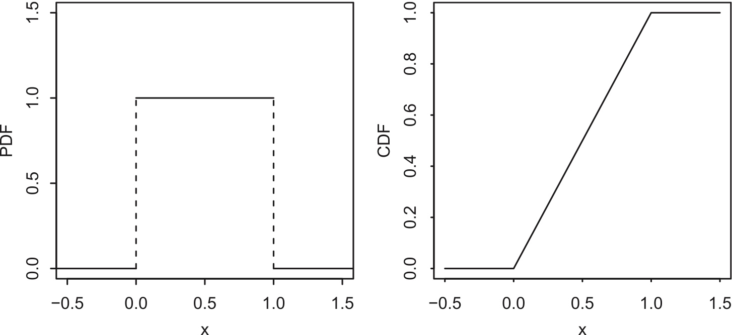
Figure 5.4: \(Unif(0, 1)\) PDF and CDF.

Proposition 5.2.2.

Let \(U\sim\mbox{Unif}(a,b)\), and let \((c, d)\) be a subinterval of \((a, b)\), of length \(l\) (so \(l=d-c\)). Then the probability of \(U\) being in \((c,d)\) is proportional to \(l\).

Proof. Since the PDF of \(U\) is the constant \(\frac{1}{b-a}\) on \((a,b)\), the area under the PDF from c to d is \(\frac{l}{b-a}\), which is a constant times \(l\).

Proposition 5.2.3. Let \(U\sim \mbox{Unif}(a,b)\), and let \((c,d)\) be a subinterval of \((a,b)\). Then the conditional distribution of \(U\) given \(U\in (c, d)\) is \(\mbox{Unif}(c, d)\).

Proof. For \(u\) in \((c, d)\), the conditional CDF at \(u\) is \[ \begin{split} P(U\leq u\mid U\in (c,d)) & = \frac{P(U\leq u,c<U<d)}{P(U\in (c,d))} \\ & = \frac{P(U\in (c,u])}{P(U\in (c,d))} \\ & = \frac{u-c}{d-c}. \end{split} \] The conditional CDF is 0 for \(u\leq c\) and 1 for \(u\geq d\). So the conditional distribution of \(U\) is as claimed.

Example 5.2.4.

• Let’s illustrate the above propositions for \(U\sim\mbox{Unif}(0, 1)\). In this special case, the support has length 1, so probability is length: the probability of \(U\) falling into the interval \((0,0.3)\) is 0.3, as is the probability of falling into \((0.3,0.6)\), \((0.4,0.7)\), or any other interval of length 0.3 within \((0,1)\).
• Now suppose that we learn that \(U\in (0.4,0.7)\). Given this information, the conditional distribution of \(U\) is \(\mbox{Unif}(0.4,0.7)\). Then the conditional probability of \(U\in (.4,.6)\) is \(2/3\), since \((0.4,0.6)\) provides \(2/3\) of the length of \((0.4,0.7)\). The conditional probability of \(U \in (0, 0.6)\) is also \(2/3\), since we discard the points to the left of 0.4 when conditioning on \(U\in(0.4,0.7)\).

Mean and variance of \(U\sim \mbox{Unif}(a,b)\) \[ E[X] = \int_a^b x f(x)\,dx = \int_a^b x \cdot \frac{1}{b - a}\,dx = \frac{1}{b - a}\cdot\frac{x^2}{2}\Big|_a^b = \frac{b^2 - a^2}{2(b - a)} = \frac{a + b}{2} \]

Use alternative formula to obtain variance: \[ \text{Var}(X) = E[X^2] - (E[X])^2 \]

\[ E[X^2] = \frac{1}{b - a}\int_a^b x^2\,dx = \frac{1}{b - a}\cdot\frac{x^3}{3}\Big|_a^b = \frac{b^3 - a^3}{3(b - a)} = \frac{b^2 + ab + a^2}{3} \]

\[ \text{Var}(X) = \frac{b^2 + ab + a^2}{3} - \left(\frac{a + b}{2}\right)^2 = \frac{(b - a)^2}{12} \]

Use definition method to obtain variance: $$ \[\begin{split} Var(X) &=\int_a^b (x-\frac{a+b}{2})^2 f(x)\,dx \\ &=\frac{1}{b - a} \int_a^b \left(x - \frac{a + b}{2}\right)^2 dx \\ &= \frac{1}{b - a} \int_a^b \left[ x^2 - (a + b)x + \frac{(a + b)^2}{4} \right] dx \\ &= \frac{1}{b - a} \left[ \frac{b^3 - a^3}{3} - (a + b)\frac{b^2 - a^2}{2} + \frac{(a + b)^2}{4}(b - a) \right]\\ &= \frac{(b - a)^2}{12} \end{split}\]

$$

Location-scale transformation

• Shifting and scaling a Uniform r.v. produces another Uniform r.v. Shifting is considered a change of location and scaling is a change of scale, hence the term location-scale.
• For example, if \(X\) is Uniform on the interval \((1, 2)\), then \(X+5\) is Uniform on the interval \((6,7)\), \(2X\) is Uniform on the interval \((2,4)\), and \(2X+5\) is Uniform on \((7,9)\).

\[ \mbox{Unif}(1, 2) \overset{X+5}{\rightarrow} \mbox{Unif}(6, 7) \]

\[ \mbox{Unif}(1, 2) \overset{2X}{\rightarrow} \mbox{Unif}(2, 4) \]

\[ \mbox{Unif}(1, 2) \overset{2X+5}{\rightarrow} \mbox{Unif}(7, 9) \]

Definition 5.2.5 (Location-scale transformation).

Let \(X\) be an r.v. and \(Y = \sigma X+\mu\), where \(\sigma\) and \(\mu\) are constants with \(\sigma > 0\). Then we say that \(Y\) has been obtained as a location-scale transformation of \(X\). Here \(\mu\) controls how the location is changed and \(\sigma\) controls how the scale is changed.

Location-scale transformation will not change distribution family, if it’s uniform, it’s still a uniform after transformation, but the parameters changed.

In the transformation \[ Y=\sigma X+\mu \] scale transform takes place first, then location transform later.

Biohazard 5.2.6.

• In a location-scale transformation, starting with \(X\sim \mbox{Unif}(a,b)\) and transforming it to \(Y=cX+d\) where \(c\) and \(d\) are constants with \(c>0\), \(Y\) is a linear function of \(X\) and Uniformity is preserved: \(Y\sim\mbox{Unif}(ca+d,cb+d)\).

• But if \(Y\) is defined as a nonlinear transformation of \(X\), then \(Y\) will not be linear in general. For example, for \(X\sim\mbox{Unif}(a,b)\) with \(0\leq a<b\), the transformed r.v. \(Y=X^2\) has support \((a^2, b^2)\) but is not Uniform on that interval. Chapter 8 explores transformations of r.v.s in detail.

• In studying Uniform distributions, a useful strategy is to start with an r.v. that has the simplest Uniform distribution, figure things out in the friendly simple case, and then use a location-scale transformation to handle the general case.

• Let’s see how this works for finding the expectation and variance of the \(\mbox{Unif}(a,b)\) distribution. The location-scale strategy says to start with \(U\sim\mbox{Unif}(0, 1)\). This is called the Standard Uniform Distribution.

  For standard uniform distribution, \[ f(x)=\left\{ \begin{array}{ll} 1 & \mbox{if}\;\; 0<x<1 \\ 0 & \mbox{otherwise}. \end{array} \right. \] and \[ F(x)=\left\{ \begin{array}{ll} 0 & \mbox{if} \;\; x\leq 0 \\ x & \mbox{if}\;\; 0<x<1 \\ 1 & x\geq 1. \end{array} \right. \]

Given that \[ X\sim \mbox{Unif}(a, b), \] how to transform it into \(Y\sim \mbox{Unif}(0, 1)\). \[ Y=\frac{X-a}{b-a} \]

During the transform from general uniform distribution to a standard unifrom, we change the location first and then scale later.

Now, given a standard uniform distribution \[ Y\sim \mbox{Unif}(0, 1) \] How to obtain a general uniform distribution \(\mbox{Unif}(a, b)\)?

We just need to reverse the steps previously.

Now, scaling first, \(Y\times (b-a)\) and plus \(a\) later.

Reverse of the transform \[ Y=\frac{X-a}{b-a} \]

\[ X=Y\times (b-a)+a \]

• The technique of location-scale transformation will work for any family of distributions such that shifting and scaling an r.v. whose distribution in the family produces another r.v. whose distribution is in the family.
• This technique does not apply to families of discrete distributions (with a fixed support) since, for example, shifting or scaling \(X\sim \mbox{Bin}(n,p)\) changes the support and produces an r.v. that is no longer Binomial. A Binomial r.v. must be able to take on all integer values between 0 and some upper bound, but \(X+4\) can’t take on any value in \(\{0, 1, 2, 3\}\) and \(2X\) can only take even values, so neither of these r.v.s has a Binomial distribution.

Biohazard 5.2.7 (Beware of sympathetic magic).

• When using location-scale transformations, the shifting and scaling should be applied to the random variables themselves, not to their PDFs. To confuse these two would be an instance of sympathetic magic and would result in invalid PDFs.

• For example, let \(U\sim\mbox{Unif}(0, 1)\), so the PDF \(f\) has \(f(x)=1\) on \((0, 1)\) (and \(f(x)=0\) elsewhere). Then \(3U+1\sim \mbox{Unif}(1, 4)\), but \(3f+1\) is the function that equals 4 on \((0, 1)\) and 1 elsewhere, which is not a valid PDF since it does not integrate to 1.

5.3 Probability integral transform

Theorem 5.3.1 (Probability Integral Transform).

Use CDF as the transformation function

Let \(F\) be a CDF which is a continuous function and strictly increasing on the support of the distribution. This ensures that the inverse function \(F^{-1}\) exists, as a function from \((0, 1)\) to \(\mathbb{R}\). We then have the following results.

1. Let \(X\) be an r.v. with CDF \(F\). Then \(F(X)\sim\mbox{Unif}(0, 1)\).
2. Let \(U\sim\mbox{Unif}(0, 1)\) and \(X=F^{-1}(U)\). Then \(X\) is an r.v. with CDF \(F\).

Proof:

1. Let \(X\) have CDF \(F\) , and find the CDF of \(Y=F(X)\). Since \(Y\) takes values in \((0, 1)\), \(P(Y\leq y)\) equals 0 for \(y\leq 0\) and equals 1 for \(y\geq 1\). For \(y\in (0, 1)\),

\[ P(Y\leq y)=P(F(X)\leq y)=P(X\leq F^{-1}(y))=F(F^{-1}(y))=y. \]

Thus \(Y\) has the \(\mbox{Unif}(0,1)\) CDF.

2. Let \(U\sim \mbox{Unif}(0, 1)\) and \(X=F^{-1}(U)\). For all real \(x\),

\[ P(X\leq x)=P(F^{-1}(U)\leq x)=P(U\leq F(x))=F(x), \]

so the CDF of \(X\) is \(F\) , as claimed. For the last equality, we used the fact that \(P(U\leq u)=u\) for \(u\in (0,1)\).

Example 5.3.3 (Percentiles).

A large number of students take a certain exam, graded on a scale from 0 to 100. Let \(X\) be the score of a random student. Continuous distributions are easier to deal with here, so let’s approximate the discrete distribution of scores using a continuous distribution. Suppose that \(X\) is continuous, with a CDF \(F\) that is strictly increasing on \((0,100)\). In reality, there are only finitely many students and only finitely many possible scores, but a continuous distribution may be a good approximation. Suppose that the median score on the exam is 60, i.e., half of the students score above 60 and the other half score below 60 (a convenient aspect of assuming a continuous distribution is that we don’t need to worry about how many students had scores equal to 60). That is, \(F(60)=1/2\), or, equivalently, \(F^{-1}(1/2)=60\).

• If Fred scores a 72 on the exam, then his percentile is the fraction of students who score below a 72. This is \(F(72)\), which is some number in \((1/2,1)\) since 72 is above the median. In general, a student with score \(x\) has percentile \(F(x)\).

• Going the other way, if we start with a percentile, say 0.95, then \(F^{-1}(0.95)\) is the score that has that percentile. A percentile is also called a quantile, which is why \(F^{-1}\) is called the quantile function. The function \(F\) converts scores to quantiles, and the function \(F^{-1}\) converts quantiles to scores.

• The strange operation of plugging \(X\) into its own CDF now has a natural interpretation: \(F(X)\) is the percentile attained by a random student. It often happens that the distribution of scores on an exam looks very non-Uniform. For example, there is no reason to think that \(10\%\) of the scores are between 70 and 80, even though \((70,80)\) covers \(10\%\) of the range of possible scores.

• On the other hand, the distribution of percentiles of the students is Uniform: the universality property says that \(F(X)\sim\mbox{Unif}(0, 1)\). For example, \(50\%\) of the students have a percentile of at least 0.5. Universality of the Uniform is expressing the fact that \(10\%\) of the students have a percentile between 0 and 0.1, \(10\%\) have a percentile between 0.1 and 0.2, \(10\%\) have a percentile between 0.2 and 0.3, and so on—a fact that is clear from the definition of percentile.

Example 5.3.4 (Probability integral transform with Logistic distribution).

The standard Logistic CDF is \[ F(x)=\frac{e^x}{1+e^x},\;\; x\in\mathbb{R} \]

# Sample from the standard logistic distribution

Y=rlogis(100000) #rlogis is sampling random number from logistic dist

hist(Y, freq = FALSE)

# apply Probability Integral Transform

U=plogis(Y) # plogis is the CDF of logistic dist

hist(U, freq = FALSE)

# quantile transform to transform U to Y

U=runif(100000)
Y=qlogis(U)

hist(Y, freq=FALSE)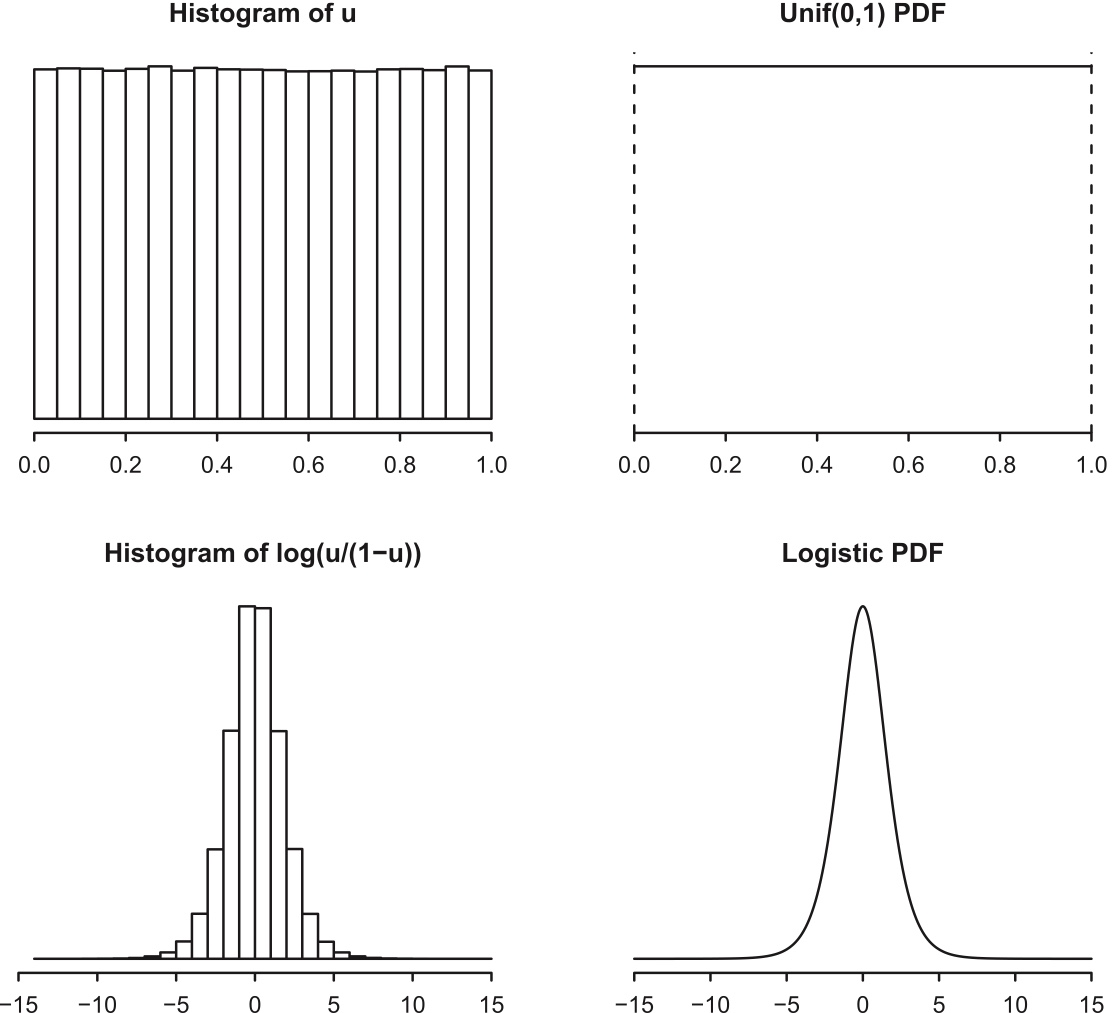

Figure 5.5: Histogram of \(10^6\) draws of \(U\sim\mbox{Unif}(0,1)\), with \(\mbox{Unif}(0, 1)\) PDF for comparison. Bottom: Histogram of \(10^6\) draws of \(\log(\frac{U}{1-U})\), with Logistic PDF for comparison.

Example 5.3.5 (Probability integral transform with Rayleigh).

The Rayleigh CDF is \[ F(x)=1-e^{-x^2/2},\;\; x>0 \] The quantile function (the inverse of the CDF) is \[ F^{-1}(u)=\sqrt{-2\log(1-u)}, \] so if \(U\sim \mbox{Unif}(0,1)\), then \(F^{-1}(U)=\sqrt{-2\log(1-U)}\sim\mbox{Rayleigh}\).

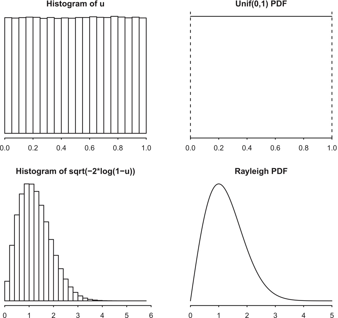
Figure 5.6: Histogram of 1 million draws from \(U\sim\mbox{Unif}(0, 1)\), with \(\mbox{Unif}(0, 1)\) PDF for comparison. Bottom: Histogram of 1 million draws from \(\sqrt{-2\log(1-U)}\), with Rayleigh PDF for comparison.

5.4 Normal distribution

The Normal distribution is a famous continuous distribution with a bell-shaped PDF. It is extremely widely used in statistics because of a theorem, the central limit theorem, which says that under very weak assumptions, the sum of a large number of i.i.d. random variables has an approximately Normal distribution, regardless of the distribution of the individual r.v.s. This means we can start with independent r.v.s from almost any distribution, discrete or continuous, but once we add up a bunch of them, the distribution of the resulting r.v. looks like a Normal distribution.

Definition 5.4.1 (Standard Normal distribution).

A continuous r.v. \(Z\) is said to have the standard Normal distribution if its PDF \(\varphi\) is given by \[ \varphi(z)=\frac{1}{\sqrt{2\pi}}e^{-z^2/2},\;\;-\infty <z <\infty. \] We write this as \(Z\sim {\cal N} (0,1)\) since, as we will show, \(Z\) has mean 0 and variance 1.

The standard Normal CDF \(\Phi\) is the accumulated area under the PDF: \[ \Phi(z)=\int_{-\infty}^z\varphi(t)dt=\int_{-\infty}^z \frac{1}{\sqrt{2\pi}}e^{-t^2/2}dt. \] It turns out to be mathematically impossible to find a closed-form expression for the antiderivative of \(\varphi\), meaning that we cannot express \(\Phi\) as a finite sum of more familiar functions like polynomials or exponentials.

Notation 5.4.2.

We can tell the Normal distribution must be special because the standard Normal PDF and CDF get their own Greek letters. By convention, we use \(\varphi\) for the standard Normal PDF and \(\Phi\) for the CDF. We will often use \(Z\) to denote a standard Normal random variable.

The PDF is bell-shaped and symmetric about 0, and the CDF is S-shaped. These have the same general shape as the Logistic PDF and CDF, but the Normal PDF decays to 0 much more quickly: notice that nearly all of the area under \(\varphi\) is between -3 and 3, whereas we had to go out to -5 and 5 for the Logistic PDF.

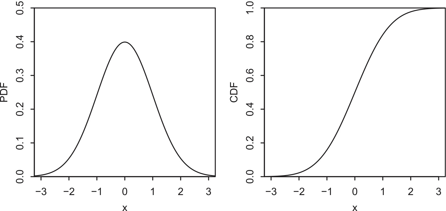
Figure 5.7: Standard Normal PDF \(\varphi\) (left) and CDF \(\Phi\) (right).

There are several important symmetry properties that can be deduced from the standard Normal PDF and CDF.

1. symmetry of PDF : \(\varphi\) satisfies \(\varphi(z)=\varphi(-z)\), i.e., \(\varphi\) is an even function.
2. Symmetry of tail areas: The area under the PDF curve to the left of -2, which is \(P(Z\leq -2)= \Phi(-2)\) by definition, equals the area to the right of 2, which is \(P(Z\geq 2)=1-\Phi(2)\). In general, we have

\[ \Phi(-z)=1-\Phi(z) \]

for all z. This can be seen visually by looking at the PDF curve, and mathematically by substituting \(u=-t\) below and using the fact that PDFs integrate to 1: \[ \begin{array}{lll} \Phi(-z) & = & \int_{-\infty}^{-z}\varphi(t)dt=-\int_\infty^z\varphi(-u)du=\int_z^\infty\varphi(u)du \\ & = & 1-\int_{-\infty}^z\varphi(u)du=1-\Phi(z). \end{array} \]

3. Symmetry of \(Z\) and \(-Z\): If \(Z\sim {\cal N}(0,1)\), then \(-Z\sim {\cal N}(0,1)\) as well. To see this, note that the CDF of \(-Z\) is

\[ P(-Z\leq z)=P(Z>-z)=1-\Phi(-z)=\Phi(z). \]

The general Normal distribution has two parameters, denoted \(\mu\) and \(\sigma^2\), which correspond to the mean and variance (so the standard Normal is the special case where \(\mu=0\) and \(\sigma^2=1\)). Starting with a standard Normal r.v. \(Z\sim {\cal N}(0,1)\), we can get a Normal r.v. with any mean and variance by a location-scale transformation (shifting and scaling).

Definition 5.4.3 (Normal distribution).

If \(Z\sim {\cal N}(0,1)\), then \[ X=\sigma Z+\mu \] is said to have the Normal distribution with mean \(\mu\) and variance \(\sigma^2\). We denote this by \(X\sim {\cal N}(\mu,\sigma^2)\).

For \(X\sim {\cal N}(\mu,\sigma^2)\), the standardized version of \(X\) is \[ \frac{X-\mu}{\sigma}\sim {\cal N}(0,1). \]

This process is called Standardization!

Theorem 5.4.4 (Normal CDF and PDF).

Let \(X\sim {\cal N}(\mu,\sigma^2)\). Then the CDF of \(X\) is \[ F(x)=\Phi\Bigl(\frac{x-\mu}{\sigma}\Bigr) \] and the PDF of \(X\) is \[ f(x)=\varphi\Bigl(\frac{x-\mu}{\sigma}\Bigr)\frac{1}{\sigma}. \]

\[ F(x)=P(X<x)=P(\frac{X-\mu}{\sigma}<\frac{x-\mu}{\sigma})=P(Z<\frac{x-\mu}{\sigma})=\Phi(\frac{x-\mu}{\sigma}) \]

Theorem 5.4.5 (68-95-99.7% rule).

If \(X\sim {\cal N}(\mu,\sigma^2)\), then \[ \begin{split} P(|X-\mu|<\sigma) & \approx 0.68 \\ P(|X-\mu|<2\sigma) & \approx 0.95 \\ P(|X-\mu|<3\sigma) & \approx 0.997. \\ \end{split} \] Often it is easier to apply the rule after standardizing, in which case we have \[ \begin{split} P(|Z|<1) & \approx 0.68 \\ P(|Z|<2) & \approx 0.95 \\ P(|Z|<3) & \approx 0.997. \\ \end{split} \]

Example 5.4.6.

Let \(X\sim {\cal N}(-1,4)\) . What is \(P(|X|<3)\), exactly (in terms of \(\Phi\)) and approximately? \[ \sigma^2=4 \]

\[ \sigma=2 \]

Do not directly do standardization inside of the absolute value sign \[ P(|X|<3)=P\left(\left|\frac{X-(-1)}{2}\right|<\frac{3-(-1)}{2}\right) \]

Instead, expand the absolute value sign, \[ P(|X|<3)=P(-3<X<3)=P(-1<\frac{X+1}{2}<2)=P(-1<Z<2)=\Phi(2)-\Phi(-1) \]

Example 5.4.7 (Folded Normal).

Let \(Y=|Z|\) with \(Z\sim N(0,1)\). The distribution of Y is called a Folded Normal with parameters \(\mu=0\) and \(\sigma^2=1\). In this example, we will derive the mean, variance, and distribution of \(Y\).

Recall: LOTUS and alternative method to obtain variance and application of CDF in the calculation of probability

\[ \begin{split} E(Y)&=\int_{-\infty}^\infty |z|f(z)dz=2\int_0^\infty |z|f(z)dz \\ &= 2\int_0^\infty z\frac{1}{\sqrt{2\pi}}e^{-z^2/2}dz \\ &= \int_0^\infty 2z\frac{1}{\sqrt{2\pi}}e^{-z^2/2}dz \\ &= 2\frac{1}{\sqrt{2\pi}}\int_0^\infty e^{-z^2/2}d(z^2/2) \\ &= 2\frac{1}{\sqrt{2\pi}}\int_0^\infty e^{-u}du \\ &= 2\frac{1}{\sqrt{2\pi}}(0-(-1))\\ &=\sqrt{\frac{2}{\pi}} \end{split} \]

\[ Var(Y)=E(Y^2)-(E(Y))^2 \]

\[ E(Y^2)=E(|Z|^2)=E(Z^2)=Var(Z)+E^2(Z)=1+0=1 \]

Thus, \[ Var(Y)=1-\frac{2}{\pi} \]

We only derive on the support of Y, which is \([0, \infty]\) \[ P(Y<y)=P(|Z|<y)=P(-y<Z<y)=\Phi(y)-\Phi(-y)=\Phi(y)-(1-\Phi(y))=2\Phi(y)-1 \]

5.5 Exponential distribution

The Exponential distribution is the continuous counterpart to the Geometric distribution. Recall that a Geometric random variable counts the number of failures before the first success in a sequence of Bernoulli trials. The story of the Exponential distribution is analogous, but we are now waiting for a success in continuous time, where successes arrive at a rate of \(\lambda\) successes per unit of time. The average number of successes in a time interval of length \(t\) is \(\lambda t\), though the actual number of successes varies randomly. An Exponential random variable represents the waiting time until the first arrival of a success.

Definition 5.5.1 (Exponential distribution).

A continuous r.v. \(X\) is said to have the Exponential distribution with parameter \(\lambda\) if its PDF is \[ f(x)=\lambda e^{-\lambda x},\;\; x>0. \] We denote this by \(X\sim\mbox{Expo}(\lambda)\). The parameter \(\lambda\) is called rate.

The corresponding CDF is \[ F(x)=1-e^{-\lambda x},\;\; x>0. \]

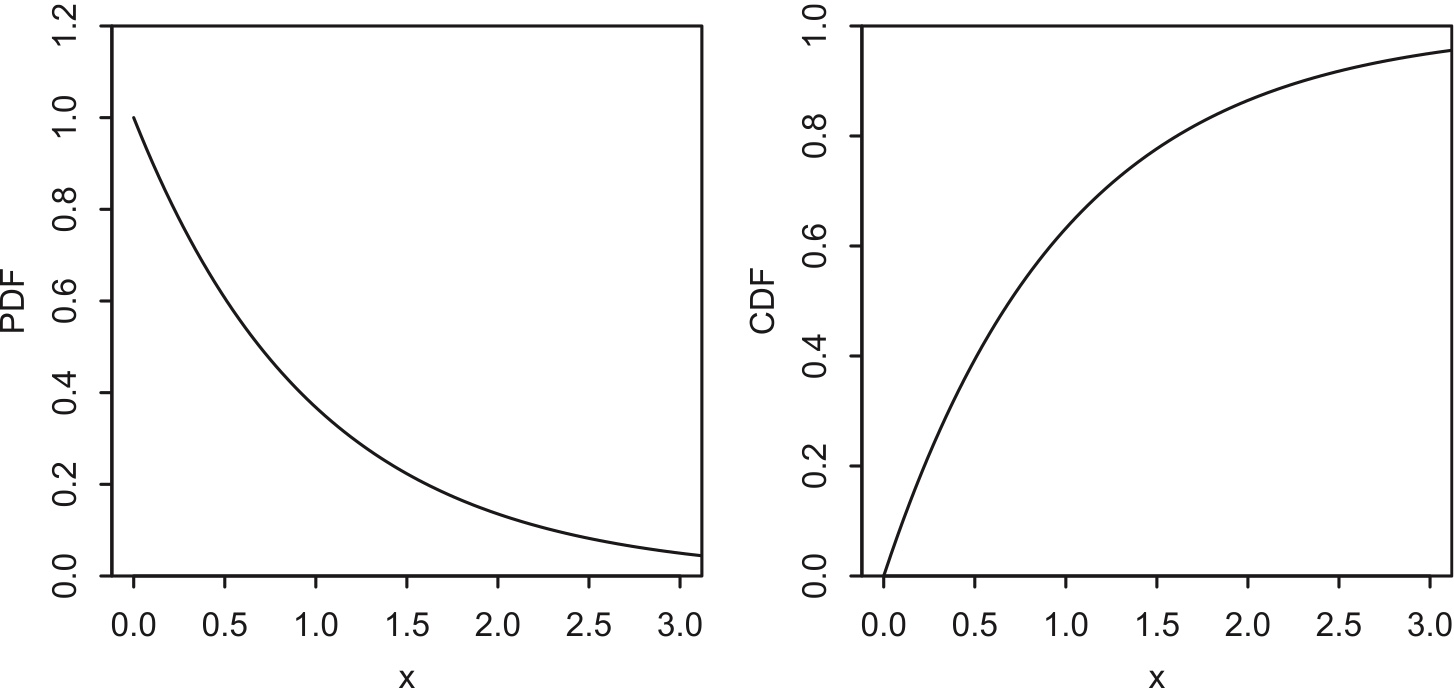
Figure 5.8: \(Expo(1)\) PDF and CDF.

• Note the resemblance to the Geometric PMF and CDF pictured in Chapter 4.

• Exponential r.v.s are defined to have support \((0,\infty)\), and shifting would change the left endpoint. But scale transformations work nicely, and we can use scaling to get from the simple Expo(1) to the general \(\mbox{Expo}(\lambda)\): if \(X\sim\mbox{Expo}(1)\), then

\[ Y=\frac{X}{\lambda}\sim \mbox{Expo}(\lambda). \]

• Conversely, if \(Y\sim\mbox{Expo}(\lambda)\), then \(\lambda Y\sim \mbox{Expo}(1)\).

Y is the waiting time with rate “\(\lambda\) occurrences / unit of time”, which means “\(\frac{1}{\lambda}\) time per occurrence”.

X is the waiting with rate “1 occurrence per unit of time”, which means “1 unit time per occurrence.” \[ P(\lambda Y < h )=P(Y< \frac{h}{\lambda})=1-e^{-\lambda (h/\lambda)}=1-e^{- h} \]

Both \(E(X)\) and \(Var(X)\) are obtained using standard integration by parts calculations. \[ \begin{split} E(X) & = \int_0^\infty xe^{-x}dx =1 \\ E(X^2) & = \int_0^\infty x^2 e^{-x}dx =2 \\ Var(X) & = E(X^2)-(EX)^2=1. \end{split} \] For \(Y = X/\lambda\sim\mbox{Expo}(\lambda)\) we then have \[ \begin{split} E(Y) & = \frac{1}{\lambda} EX =\frac{1}{\lambda}\\ Var(Y) & = \frac{1}{\lambda^2} Var(X) =\frac{1}{\lambda^2}. \end{split} \] As we’d expect intuitively, the faster the rate of arrivals \(\lambda\), the shorter the average waiting time.

The Exponential distribution has a very special property called the memoryless property, which says that even if you’ve waited for hours or days without success, the success isn’t any more likely to arrive soon. In fact, you might as well have just started waiting 10 seconds ago. The definition formalizes this idea.

Definition 5.5.2 (Memoryless property).

A distribution is said to have the memoryless property if a random variable X from that distribution satisfies \[ P(X\geq s+t\mid X\geq s)= P(X\geq t) \] for all \(s,t>0\).

Proof: \[ P(X\ge s+t\mid X\ge s)=\frac{P(X\ge s+t)}{P(X\ge s)}=\frac{1-F(s+t)}{1-F(s)}=\frac{e^{-\lambda (s+t)}}{e^{-\lambda s}}=e^{-\lambda t}=1-F(t)=P(X\ge t) \]

Here \(s\) represents the time you’ve already spent waiting; the definition says that after you’ve waited \(s\) minutes, the probability you’ll have to wait another \(t\) minutes is exactly the same as the probability of having to wait \(t\) minutes with no previous waiting time under your belt. Another way to state the memoryless property is that conditional on \(X\geq s\), the additional waiting time \(X-s\) is still distributed \(\mbox{Expo}(\lambda)\). In particular, this implies \[ E(X\mid X\geq s)=s+E(X)=s+\frac{1}{\lambda}. \]

• Using the definition of conditional probability, we can directly verify that the Exponential distribution has the memoryless property.

• What are the implications of the memoryless property? If you’re waiting at a bus stop and the time until the bus arrives has an Exponential distribution, then conditional on your having waited 30 minutes, the bus isn’t due to arrive soon. The distribution simply forgets that you’ve been waiting for half an hour, and your remaining wait time is the same as if you had just shown up to the bus stop.

• If the lifetime of a machine has an Exponential distribution, then no matter how long the machine has been functional, conditional on having lived that long, the machine is as good as new: there is no wear-and-tear effect that makes the machine more likely to break down soon.

• If human lifetimes were Exponential, then conditional on having survived to the age of 80, your remaining lifetime would have the same distribution as that of a newborn baby!

Clearly, the memoryless property is not an appropriate description for human or machine lifetimes. Why then do we care about the Exponential distribution?

1. Some physical phenomena, such as radioactive decay, truly do exhibit the memoryless property, so the Exponential is an important model in its own right.
2. The Exponential distribution is well-connected to other named distributions. In the next section, we’ll see how the Exponential and Poisson distributions can be united by a shared story, and we’ll discover many more connections in later chapters.
3. The Exponential serves as a building block for more flexible distributions, such as the Weibull distribution (see Exercise 25 of Chapter 6), that allow for a wear-and-tear effect (where older units are due to break down) or a survival-of-the-fit test effect (where the longer you’ve lived, the stronger you get). To understand these distributions, we first have to understand the Exponential.

The memoryless property is a very special property of the Exponential distribution: no other continuous distribution on \((0,\infty)\) is memoryless!

Theorem 5.5.3.

If \(X\) is a positive continuous random variable with the memoryless property, then \(X\) has an Exponential distribution.

Proof. See textbook.

In view of the analogy between the Geometric and Exponential stories, you might guess that the Geometric distribution also has the memoryless property. If so, you would be correct! If we’re waiting for the first Heads in a sequence of fair coin tosses, and in a streak of bad luck we happen to get ten Tails in a row, this has no impact on how many additional tosses we’ll need: the coin isn’t due for a Heads, nor conspiring against us to perpetually land Tails. The coin is memoryless. The Geometric is the only memoryless discrete distribution (with support \(0,1,\ldots\)), and the Exponential is the only memoryless continuous distribution (with support \((0,\infty)\)).

As practice with the memoryless property, the following example chronicles the adventures of Fred, who experiences firsthand the frustrations of the memoryless property after moving to a town with a memoryless public transportation system.

Example 5.5.4 (Blissville and Blotchville).

Fred lives in Blissville, where buses always arrive exactly on time, with the time between successive buses fixed at 10 minutes. Having lost his watch, he arrives at the bus stop at a uniformly random time on a certain day (assume that buses run 24 hours a day, every day, and that the time that Fred arrives is independent of the bus arrival process).

1. What is the distribution of how long Fred has to wait for the next bus? What is the average time that Fred has to wait?

Fred arrives uniformly between two bus arrivals, which has length fixed at \(10\) minutes. \[ \mbox{Unif}(0, 10) \] Expectation of Uniform is \(10/2=5\).

2. Given that the bus has not yet arrived after 6 minutes, what is the probability that Fred will have to wait at least 3 more minutes?

\[ P(T> 6+3 \mid T>6)=\frac{P(T>9)}{P(T>6)}=\frac{1-\frac{9}{10}}{1-\frac{6}{10}}=1/4 \]

\[ P(T>3)=1-\frac{3}{10}=7/10 \]

3. Fred moves to Blotchville, a city with inferior urban planning and where buses are much more erratic. Now, when any bus arrives, the time until the next bus arrives is an Exponential random variable with mean 10 minutes. Fred arrives at the bus stop at a random time, not knowing how long ago the previous bus came. What is the distribution of Fred’s waiting time for the next bus? What is the average time that Fred has to wait?

The mean of waiting time between two bus arrivals is \(10\), so \(1/\lambda=10\). \[ T \sim \mbox{Expo}(1/10) \]

Because Exponential distribution has memoryless property, so without knowing when the previous bus arrived, the extra waiting for Fred is still the same exponential distribution with \(\lambda=1/10\).

4. When Fred complains to a friend how much worse transportation is in Blotchville, the friend says: “Stop whining so much! You arrive at a uniform instant between the previous bus arrival and the next bus arrival. The average length of that interval between buses is 10 minutes, but since you are equally likely to arrive at any time in that interval, your average waiting time is only 5 minutes.” Fred disagrees, both from experience and from solving Part (c) while waiting for the bus. Explain what is wrong with the friend’s reasoning.

Fred’s friend is making the mistake, explained in Biohazard 4.1.3, of replacing a random variable (the time between buses) by its expectation (10 minutes), thereby ignoring the variability in interarrival times. The average length of a time interval between two buses is 10 minutes, but Fred is not equally likely to arrive at any of these intervals: Fred is more likely to arrive during a long interval between buses than to arrive during a short interval between buses. For example, if one interval between buses is 50 minutes and another interval is 5 minutes, then Fred is 10 times more likely to arrive during the 50-minute interval.

This phenomenon is known as length-biasing, and it comes up in many real-life situations.

For example,

Mothers vs. Siblings Paradox:

1. Ask mothers: “How many children do you have?”
2. Ask randomly chosen people: “How many siblings do you have (including yourself)?”

These two answers give different distributions.

Class size paradox:

Asking students the sizes of their classes and averaging those results may give a much higher value than taking a list of classes and averaging the sizes of each (this is called the class size paradox).

5.6 Gamma distribution

The Gamma distribution is a continuous distribution on the positive real line; it is a generalization of the Exponential distribution. While an Exponential r.v. represents the waiting time for the first success under conditions of memorylessness, we shall see that a Gamma r.v. represents the total waiting time for multiple successes. Before writing down the PDF, we first introduce the gamma function, a very famous function in mathematics that extends the factorial function beyond the realm of nonnegative integers.

Definition 8.4.1 (Gamma function).

The gamma function \(\Gamma\) is defined by \[ \Gamma(\alpha)=\int_0^\infty x^{\alpha-1} e^{-x}dx, \] for real numbers \(\alpha>0\).

Here are two important properties of the gamma function.

• \(\Gamma(\alpha+1)=\alpha\Gamma(\alpha)\) for all \(a>0\). This follows from integration by parts:

\[ \begin{array}{l} \Gamma(\alpha+1)=\int_0^\infty x^\alpha e^{-x} dx=-x^\alpha e^{-x}|_0^\infty +\alpha\int_0^\infty e^{-x}x^{\alpha-1}dx \\ =0+\alpha\Gamma(\alpha). \end{array} \]

• \(\Gamma(n)=(n-1)!\) if \(n\) is a positive integer. This can be proved by induction, starting with \(n=1\) and using the recursive relation \(\Gamma(\alpha+1)=\alpha\Gamma(\alpha)\). Thus, if we evaluate the gamma function at positive integer values, we recover the factorial function (albeit shifted by 1).

Now let’s suppose that on a whim, we decide to divide both sides of the above definition by \(\Gamma(a)\). We have \[ 1=\int_0^\infty \frac{1}{\Gamma(\alpha)}x^{\alpha-1}e^{-x}dx, \] so the function under the integral is a valid PDF supported on \((0,\infty)\). This is the definition of the PDF of the Gamma distribution. Specifically, we say that \(X\) has the Gamma distribution with parameters \(\alpha\) and 1, denoted \(X\sim\mbox{Gamma}(\alpha,1)\), if its PDF is \[ f_X(x)=\frac{1}{\Gamma(\alpha)}x^{\alpha-1}e^{-x},\;\; x>0. \]

From the \(\mbox{Gamma}(\alpha,1)\) distribution, we obtain the general Gamma distribution by a scale transformation: if \(X\sim\mbox{Gamma}(\alpha,1)\) and \(\lambda>0\), then the distribution of \(Y=X/\lambda\) is called the \(\mbox{Gamma}(a,\lambda)\) distribution.

• \(X\): is the waiting time for \(\alpha\) occurrences;
• \(Y=X/\lambda\): now the waiting time is the original one’s \(1/\lambda\), which means the occurrence is more frequent. In other words, the rate is increased by \(\lambda\) times.

Recalled: the scale \(\beta\) is the reciprocal of the rate, \[ \beta=\frac{1}{\lambda} \] In some literature, Gamma distributions are parameterized by the scale parameter instead of the rate, so we have \(\mbox{Gamma}(\alpha, \beta)\).

Definition 8.4.2 (Gamma distribution).

An r.v. \(Y\) is said to have the Gamma distribution with parameters \(\alpha\) and \(\lambda\), \(\alpha>0\) and \(\lambda>0\), if its PDF is \[ f(y)=\frac{\lambda^\alpha}{\Gamma(\alpha)}y^{\alpha-1}e^{-\lambda y}\;\; y>0. \] We write \(Y\sim\mbox{Gamma}(\alpha,\lambda)\).

Taking \(\alpha=1\), the \(\mbox{Gamma}(1,\lambda)\) PDF is \(f(y)=\lambda e^{-\lambda y}\) for \(y>0\), so the \(\mbox{Gamma}(1,\lambda)\) and \(\mbox{Expo}(\lambda)\) distributions are the same.

The extra parameter \(\alpha\) allows Gamma PDFs to have a greater variety of shapes.

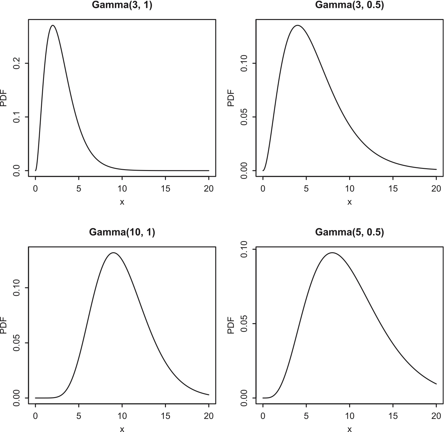
Figure 5.9: Gamma PDFs for various values of \(\alpha\) and \(\lambda\). Clockwise from top left: Gamma(3, 1), Gamma(3, 0.5), Gamma(5, 0.5), Gamma(10, 1).

Theorem 8.4.3.

Let \(X_1,\ldots,X_n\) be i.i.d. \(\mbox{Expo}(\lambda)\). Then \[ X_1+\ldots X_n\sim\mbox{Gamma}(n,\lambda). \] Thus, if \(Y\sim\mbox{Gamma}(\alpha,\lambda)\) with \(\alpha\) an integer, we can represent \(Y\) as a sum of i.i.d. \(\mbox{Expo}(\lambda)\) r.v.s, \(X_1+\ldots + X_\alpha\), and get the mean and variance right away: \[ \begin{split} E(Y) & = E(X_1+\ldots +X_\alpha)=\alpha E(X_1)=\frac{\alpha}{\lambda}, \\ \mbox{Var}(Y) & = \mbox{Var}(X_1+\ldots +X_\alpha)=\alpha \mbox{Var}(X_1)=\frac{\alpha}{\lambda^2}. \end{split} \]

Mathematically, the expectation of \(Y\) can be obtained. \[ \begin{split} E(Y)& =\int_{y=0}^\infty y\frac{\lambda^\alpha}{\Gamma(\alpha)}y^{\alpha-1}e^{-\lambda y} dy \\ &=\int_{y=0}^\infty \frac{\lambda^\alpha}{\Gamma(\alpha)}y^{\alpha}e^{-\lambda y} dy \\ &=\frac{\lambda^\alpha}{\Gamma(\alpha)}\int_{y=0}^\infty y^{\alpha}e^{-\lambda y} dy \\ &=\frac{\lambda^\alpha}{\Gamma(\alpha)}\frac{\Gamma(\alpha+1)}{\lambda^{\alpha+1}}\int_{y=0}^\infty \frac{\lambda^{\alpha+1}}{\Gamma(\alpha+1)}y^{(\alpha+1)-1}e^{-\lambda y} dy \\ &=\frac{\lambda^\alpha}{\Gamma(\alpha)}\frac{\Gamma(\alpha+1)}{\lambda^{\alpha+1}} \\ &=\frac{\alpha}{\lambda} \end{split} \]

To obtain the variance in mathematical way, we can use the alternative formula \[ Var(Y)=E(Y^2)-(E(Y))^2 \] Use the similar way to obtain \(E(Y^2)\).

5.7 Poisson-Gamma relationship

If \(X \sim \text{Gamma}(\alpha,\lambda)\) where \(\alpha\) is an integer, then for any \(x\),

\[ P(X < x) = P(Y > \alpha), \]

where \(Y \sim \text{Poisson}(\lambda x)\).

\(X\): waiting time for \(\alpha\) occurrence

\(Y\): the number of occurrence in a Poisson process with a rate \(\lambda x\).

• the $P(X < x) $ means “waiting time for \(\alpha\) occurrences is less than \(x\)”
• the \(P(Y > \alpha)\) means “the number of occurrences in the time \(x\) is more than \(\alpha\)”

We start from the Gamma CDF:

\[ P(X \le x) = \frac{ \lambda^\alpha}{(\alpha - 1)! } \int_0^x t^{\alpha - 1} e^{-\lambda t} \, dt. \]

Apply integration by parts with

\[ u = t^{\alpha - 1}, dv = e^{-\lambda t}\,dt \]

\[ P(X \le x) = -\frac{\lambda^{\alpha - 1}}{(\alpha - 1)! \, } x^{\alpha - 1} e^{-\lambda x} + \frac{\lambda^{\alpha - 1}}{(\alpha - 2)! \, } \int_{0}^{x} t^{\alpha - 2} e^{-\lambda t} \, dt. \]

Note that

\[ P(Y = \alpha - 1) = \frac{(\lambda x)^{\alpha - 1}e^{-\lambda x}}{(\alpha - 1)!}, \]

Recall :

The pmf of a Poisson random variable \(K \sim \text{Poisson}(\lambda)\) is

\[ P(K = k) = \frac{\lambda^k e^{-\lambda}}{k!}, \quad k = 0,1,2,\ldots \] What is the pdf of \(Y\sim\)Poisson\((\lambda x)\) \[ P(Y = k) = \frac{(\lambda x)^k e^{-\lambda x}}{k!}, \quad k = 0,1,2,\ldots \]

so the boundary term becomes \[ -\frac{\lambda^{\alpha - 1}}{(\alpha - 1)! \, } x^{\alpha - 1} e^{-\lambda x} = -P(Y = \alpha - 1). \]

Thus,

\[ P(X \le x) = \frac{\lambda^{\alpha - 1}}{(\alpha - 2)! \, } \int_0^x t^{\alpha - 2} e^{-\lambda t} \, dt - P(Y = \alpha - 1). \]

Since \(P(Y = \alpha - 1) = 1 - P(Y \ge \alpha - 1)\), repeated integration by parts eventually yields:

\[ P(X < x) = P(Y > \alpha). \]

5.8 Transformation of r.v.

Given r.v. \(X\) which has probability density function \(f(x)\), what is the pdf of \[ Y=g(X) \] where \(g\) is a transformation function?

If \(g\) is the cdf of \(X\), we know that is called probability integral transform, and \(Y\) will have standard uniform distribution.

For other cases of \(g\), we need to discuss.

If \(g\) is differentiable and strictly increasing or strictly decreasing, then the PDF of Y is given by \[ f_Y(y)=f_X(x)\left |\frac{dx}{dy}\right| \] where \(x=g^{-1}(y)\).