Chapter 3 Ch. 3: Random Variables and Their Distributions
3.1 Random variables
Definition 3.1.1 (Random variable).
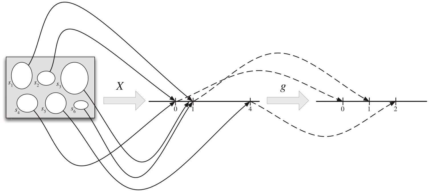
Given an experiment with sample space \(S\), a random variable (r.v.) is a function from the sample space \(S\) to the real numbers \(\mathbb{R}\). It is common, but not required, to denote random variables by capital letters.
Thus, a random variable \(X\) assigns a numerical value \(X(s)\) to each possible outcome \(s\) of the experiment. The randomness comes from the fact that we have a random experiment (with probabilities described by the probability function \(P\)).
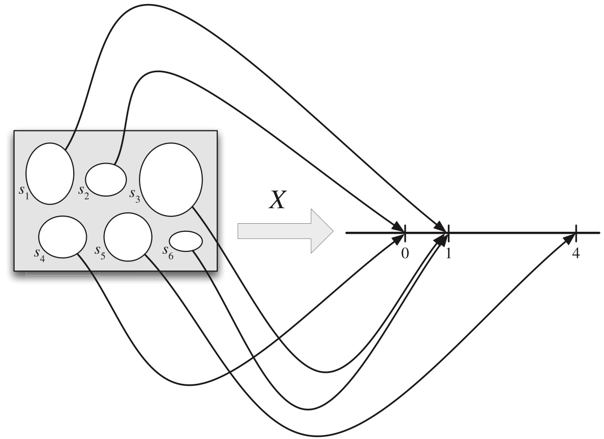
Figure 3.1: A random variable maps the sample space into the real line. The r.v. X depicted here is defined on a sample space with 6 elements, and has possible values 0, 1, and 4.
Since random variable is a function,
multiple outcomes from the sample space can be mapped to the same real number, (in Figure 3.1, \(s_1\), \(s_3\), and \(s_6\) are all mapped to \(1\)).
the same outcome cannot be assigned to different real numbers.
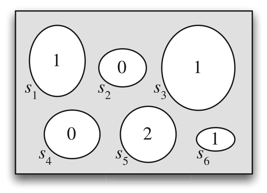
multiple random variables can be defined on the same sample space, just like multiple functions can be defined on the same domain. In Figure 3.2, two different random variables are defined on the same sample space.
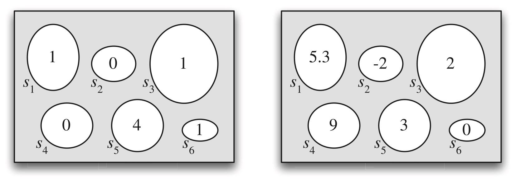
Figure 3.2: Two random variables defined on the same sample space.
Summary:
- random variable is a function, encoding random outcomes into real numbers;
- informally, you may interpret values of random variables as codes for random outcomes;
- you may also interpret random outcomes as labels for the values of random variables;
For example:
| Random outcomes | Values of Random variable |
|---|---|
| Freshmen | 1 |
| Sophomore | 2 |
| Junior | 3 |
| Senior | 4 |
| Master | 5 |
| Phd | 6 |
Mutiple outcomes can be asigned to the same value of randome variable:
| Random outcomes | Values of Random variable |
|---|---|
| Freshmen, Sophomore, Junior, Senior | 1 |
| Master or Phd | 2 |
Example 3.1.2 (Coin tosses).
Consider an experiment where we toss a fair coin twice. The sample space consists of four possible outcomes: \(S = \{HH, HT, TH, TT\}\). Here are some random variables on this space (for practice, you can think up some of your own). Each r.v. is a numerical summary of some aspect of the experiment.
Let \(X\) be the number of Heads. This is a random variable with possible values 0, 1, and 2. Viewed as a function, \(X\) assigns the value 2 to the outcome \(HH\), 1 to the outcomes \(HT\) and \(TH\), and 0 to the outcome \(TT\). That is,
\[ X(HH) = 2, \quad X(HT) = X(TH) = 1, \quad X(TT) = 0. \]
Let \(Y\) be the number of Tails. In terms of \(X\), we have \(Y = 2 - X\). In other words, \(Y\) and \(2 - X\) are the same r.v.:
\[ Y(s) = 2 - X(s) \quad \text{for all } s. \]Let \(I\) be 1 if the first toss lands Heads and 0 otherwise. Then \(I\) assigns the value 1 to the outcomes \(HH\) and \(HT\), and 0 to the outcomes \(TH\) and \(TT\). This r.v. is an example of what is called an indicator random variable since it indicates whether the first toss lands Heads, using 1 to mean “yes” and 0 to mean “no”.
3.2 Types of random variables
There are two main types of random variables used in practice: ==discrete== r.v.s and ==continuous== r.v.s. In this chapter and the next, our focus is on discrete r.v.s. Continuous r.v.s are introduced in Chapter 5.
Definition (Discrete random variable). A random variable \(X\) is said to be discrete if
there is a finite number of possible values that \(X\) can take, or there is a ==countably infinite number== of possible values that \(X\) can take.
Example of countably infinite: Natrual numbers, Integer numbers, etc.
Distcrete random variables can only take some possible values in an interval, such as integers;
Continuous random variables can take all possible values in an interval, such as all numbers betwen \(0\) to \(1\).
If \(X\) is a discrete r.v., then the finite or countably infinite set of values \(x\) such that \(P (X = x) > 0\) is called the support of \(X\).
Most commonly in applications, the support of a discrete r.v. is a set of integers. In contrast, a continuous r.v. can take on any real value in an interval (possibly even the entire real line).
3.3 Probability mass functions (PMF)
Definition 3.2.2 (Probability mass function).
The probability mass function (PMF) of a discrete r.v. \(X\) is the function \(p_X\) given by \(p_X (x) = P (X = x)\). Note that this is positive if \(x\) is in the support of \(X\), and 0 otherwise.
In writing \(P (X = x)\), we are using \(X = x\) to denote an event, consisting of all outcomes \(s\) to which \(X\) assigns the number \(x\). This event is also written as \(\{X = x\}\); formally, \(\{X = x\}\) is defined as \(\{s \in S : X(s) = x\}\), but writing \(\{X = x\}\) is shorter and more intuitive.
PMF describes the probability of the random variable \(X\) takes a specific value, \[ p_X(x)=P(X\text{ takes the value }x). \] The capitalized \(X\) is a random variable, and the lower case \(x\) is specific number, such as \(1\).
\[ P(X=1)=P(\text{X takes the value 1})=p_X(1) \] Summary:
PMF \(p_X\) is a function
\(p_X\) takes possible values of a random variable \(X\) and return a probability of \(X\) taking that value;
a possible value that the random variable can take is usually denoted by a lowercase letter, such as \(x\)
a random variable itself, as a function, is often denoted by a captilized letter, such as \(X\)
You must distinguish between possible values of a random variable and the random variable itself.
\(X\) is the random variable itself, which is a function; \(x\) is a possible value of the random variable \(X\).
The input of PMF \(p_X\) is a possible value of the random variable \(X\), NOT the random variable itself!
==What is the domain of a PMF?==
The domain of a PMF is always \((-\infty, \infty)\)!
But we know that a discrete random variable \(X\) can only take some values in the real number. For these values, the PMF \(P(X=x)\) is greater than \(0\). For other values, the probability \(P(X=x)=0\).
The support of a PMF is the set of values that \(X\) can possibly take. By “can possibly take”, we mean the probability of \(X\) taking those values is greater than zero.
Example 3.2.4 (Coin tosses continued).
In this example we’ll find the PMFs of all the random variables in Example 3.1.2, the example with two fair coin tosses. Here are the r.v.s we defined, along with their PMFs:
\(X\), the number of Heads. Since \(X\) equals 0 if \(TT\) occurs, 1 if \(HT\) or \(TH\) occurs, and 2 if \(HH\) occurs,
the PMF of \(X\) is the function \(p_X\) given by \[ p_X(0) = P(X = 0) = \tfrac{1}{4}, \\ p_X(1) = P(X = 1) = \tfrac{1}{2}, \\ p_X(2) = P(X = 2) = \tfrac{1}{4}, \]and \(p_X(x) = 0\) for all other values of \(x\).
For example, \(p_X(3)=0\). \(p_X\) is defined at \(3\), however, the value of \(p_X(3)\) is zero. So \(3\) is not in the support of \(p_X\). The support of \(p_X\) is \((0, 1, 2)\), for which \(p_X\) returns non-zero probabilities.
The support of a PMF is the collection of values that the random variable can possibly take. In other words, the evaluation of PMF on the support returns nonzero probability.
\(Y = 2 - X\), the number of Tails. Reasoning as above or using the fact that \[ P(Y = y) = P(2 - X = y) = P(X = 2 - y) = p_X(2 - y), \]
the PMF of \(Y\) is
\[ p_Y(0) = P(Y = 0) = \tfrac{1}{4}, \\ p_Y(1) = P(Y = 1) = \tfrac{1}{2}, \\ p_Y(2) = P(Y = 2) = \tfrac{1}{4}, \]
and \(p_Y(y) = 0\) for all other values of \(y\).
\(I\), the indicator of the first toss landing Heads. Since \(I\) equals 0 if \(TH\) or \(TT\) occurs and 1 if \(HH\) or \(HT\) occurs, the PMF of \(I\) is \[ p_I(0) = P(I = 0) = \tfrac{1}{2}, \\ p_I(1) = P(I = 1) = \tfrac{1}{2}, \]
and \(p_I(i) = 0\) for all other values of \(i\).
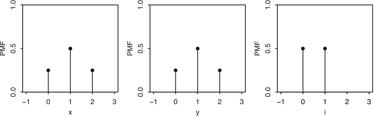
Figure 3.3: Left to right: PMFs of \(X\), \(Y\) , and \(I\), with \(X\) the number of Heads in two fair coin tosses, \(Y\) the number of Tails, and \(I\) the indicator of Heads on the first toss.
Example 3.2.5 (Sum of die rolls).
We roll two fair 6-sided dice. Let \(T = X + Y\) be the total of the two rolls, where \(X\) and \(Y\) are the individual rolls. The sample space of this experiment has 36 equally likely outcomes: \[ S=\{(1,1),(1,2),\ldots,(6,5),(6,6)\}. \]
| Y=1 | Y=2 | Y=3 | Y=4 | Y=5 | Y=6 | |
|---|---|---|---|---|---|---|
| X=1 | (1, 1) | (1, 2) | (1, 3) | (1, 4) | (1, 5) | (1, 6) |
| X=2 | (2, 1) | (2, 2) | (2, 3) | (2, 4) | (2, 5) | (2, 6) |
| X=3 | (3, 1) | (3, 2) | (3, 3) | (3, 4) | (3, 5) | (3, 6) |
| X=4 | (4, 1) | (4, 2) | (4, 3) | (4, 4) | (4, 5) | (4, 6) |
| X=5 | (5, 1) | (5, 2) | (5, 3) | (5, 4) | (5, 5) | (5, 6) |
| X=6 | (6, 1) | (6, 2) | (6, 3) | (6, 4) | (6, 5) | (6, 6) |
| T = X + Y | Y=1 | Y=2 | Y=3 | Y=4 | Y=5 | Y=6 |
|---|---|---|---|---|---|---|
| X=1 | 2 | 3 | 4 | 5 | 6 | 7 |
| X=2 | 3 | 4 | 5 | 6 | 7 | 8 |
| X=3 | 4 | 5 | 6 | 7 | 8 | 9 |
| X=4 | 5 | 6 | 7 | 8 | 9 | 10 |
| X=5 | 6 | 7 | 8 | 9 | 10 | 11 |
| X=6 | 7 | 8 | 9 | 10 | 11 | 12 |
The random variable \(T\) may take possible values \(\{2, 3, 4, 5, 6, 7, 8, 9, 10, 11, 12\}\).
- By the naive definition of probability,
\[ \begin{split} P(T=2) &= P(T=12)=1/36 \\ P(T=3) &= P(T=11)=2/36 \\ P(T=4) &= P(T=10)=3/36 \\ P(T=5) &= P(T=9)=4/36 \\ P(T=6) &= P(T=8)=5/36 \\ P(T=7) &= 6/36. \end{split} \]
- For all other values of \(t\), \(P(T=t)=0\).
- The support of \(T\) is \(\{2,3,\ldots,12\}\).
- \(P(T=2)+P(T=3)+\ldots +P(T=12)=1\).
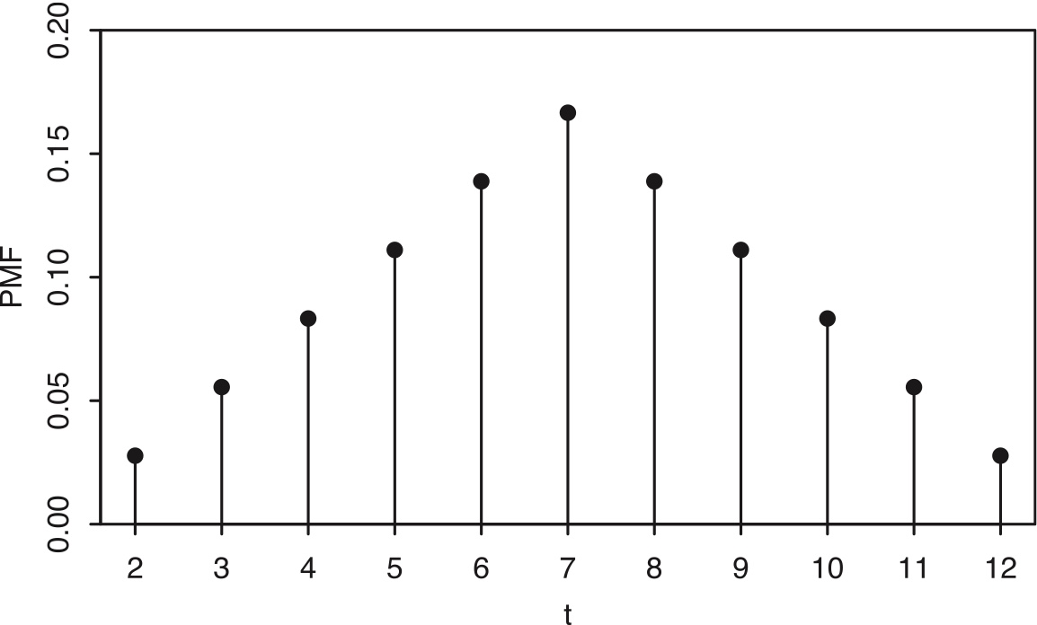
Figure 3.4: PMF of the sum of two die rolls.
Example 3.2.6 (Children in a U.S. household).
Suppose we choose a household in the United States at random. Let \(X\) be the number of children in the chosen household. Since \(X\) can only take on integer values, it is a discrete r.v. The probability that \(X\) takes on the value \(x\) is proportional to the number of households in the United States with \(x\) children. Using data from the 2010 General Social Survey, we can approximate the proportion of households with 0 children, 1 child, 2 children, etc., and hence approximate the PMF of \(X\), which is plotted on the next page.
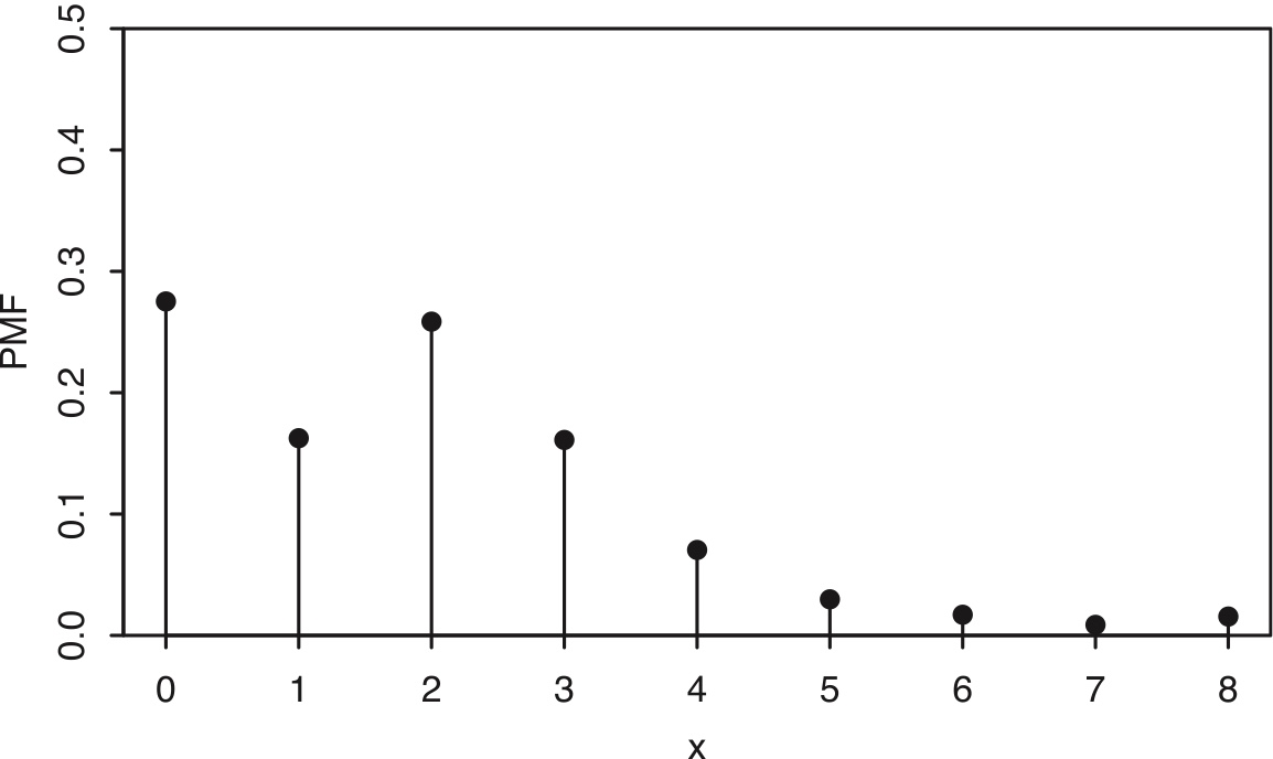
Figure 3.5: PMF of the number of children in a randomly selected U.S. household.
Theorem 3.2.7 (Valid PMFs).
Let \(X\) be a discrete r.v. with support \(x_1, x_2,\ldots\) (assume these values are distinct and, for notational simplicity, that the support is countably infinite; the analogous results hold if the support is finite). The PMF \(p_X\) of \(X\) must satisfy the following two criteria:
- Nonnegative: \(p_X(x)>0\) if \(x=x_j\) for some \(j\), and \(p_X(x)=0\) otherwise;
- Sums to 1: \({\displaystyle \sum_{j=1}^\infty p_X(x_j)=1}\).
Example 3.2.8. Application of PMF
Returning to Example 3.2.5, let \(T\) be the sum of two fair die rolls. We have already calculated the PMF of \(T\) . Now suppose we’re interested in the probability that \(T\) is in the interval \([1, 4]\). There are only three values in the interval \([1, 4]\) that \(T\) can take on, namely, 2, 3, and 4. We know the probability of each of these values from the PMF of \(T\) , so \[ P(1\leq T\leq 4)=P(T=2)+P(T=3)+P(T=4)=\frac{6}{36}. \]
- In general, given a discrete r.v. \(X\) and a set \(B\) of real numbers, if we know the PMF of \(X\) we can find \(P (X\in B)\), the probability that \(X\) is in \(B\), by summing up the heights of the vertical bars at points in \(B\) in the plot of the PMF of \(X\). Knowing the PMF of a discrete r.v. determines its distribution.
3.4 Bernoulli trial
An experiment that can result in two possible outcomes, either a “success” or a “failure” (but not both) is called a Bernoulli trial.
In this context, the outcomes are referred to as “success” or “failure” in a generic sense. As long as the outcomes are binary, the random experiment qualifies as a Bernoulli trial.
For example, if we flip a coin, there are two possible outcomes: Head or Tail, so this is a Bernoulli trial.
Suppose we draw balls with replacement from a container containing white and black balls. Each draw can result in either a white ball or a black ball — a binary outcome. Therefore, each draw represents a Bernoulli trial.
3.5 Bernoulli distribution
In a Bernoulli trial, we can encode the two possible outcomes as \(0\) and \(1\), such as
- \(success=1\)
- \(failure=0\).
So the random variable is defined as
\[ X(outcome) = \left\{ \begin{array}{rl} 1 & \mbox{if outcome is success} \\ 0 & \mbox{if outcome is failure} \end{array}\right. \] The Bernoulli random variable \(X\) can be thought of as the indicator of success in a Bernoulli trial: it equals \(1\) if success occurs and \(0\) if failure occurs in the trial.
In a Bernoulli trial the the success probability is often denoted as \(p\), which is the probability of \(X\) taking the value \(1\), \[ P(X=1)=p. \] For example, if we flip a fair coin, the probability of getting a head (success) is \(0.5\), so \(p=0.5\).
If a random variable \(X\) is defined as the indicator of success in a Bernoulli trial, its probability distribution is called Bernoulli distribution.
Definition 3.3.1 (Bernoulli distribution).
A r.v. \(X\) is said to have the Bernoulli distribution with parameter \(p\) if \(P(X=1)=p\) and \(P(X=0)=1-p\), where \(0<p<1\). We write this as \(X\sim\mbox{Bern}(p)\). The symbol \(\sim\) is read ``is distributed as’’.
Definition 3.3.2 (Indicator random variable).
The indicator random variable of an event \(A\) is the r.v. which equals 1 if \(A\) occurs and 0 otherwise. We will denote the indicator r.v. of \(A\) by \(I_A\) or \(I(A)\). Note that \(I_A \sim \mbox{Bern(p)}\) with \(p = P (A)\).
3.6 Binomial distribution
Suppose that \(n\) independent Bernoulli trials are performed, each with the same success probability \(p\).
Let \(X\) be the number of successes. The distribution of \(X\) is called the Binomial distribution with parameters \(n\) and \(p\). We write \(X \sim Bin(n, p)\) to mean that \(X\) has the Binomial distribution with parameters \(n\) and \(p\), where \(n\) is a positive integer and \(0 < p < 1\).
Theorem 3.3.5 (Binomial PMF).
If \(X \sim \mbox{Bin}(n, p)\), then the PMF of \(X\) is \[ P(X=k)={n\choose k}p^k(1-p)^{n-k} \] for \(k=0,1,\ldots,n\) (and \(P(X=k)=0\) otherwise).
To save writing, it is often left implicit that a PMF is zero wherever it is not specified to be nonzero, but in any case it is important to understand what the support of a random variable is, and good practice to check that PMFs are valid. If two discrete r.v.s have the same PMF, then they also must have the same support.
Proof. An experiment consisting of \(n\) independent Bernoulli trials produces a sequence of successes and failures. The probability of any specific sequence of \(k\) successes and \(n-k\) failures is \(p^k(1-p)^{n-k}\). There are \({n\choose k}\) such sequences, since we just need to select where the successes are. Therefore, letting \(X\) be the number of successes,
\[ P(X=k)={n\choose k}p^k(1-p)^{n-k} \] for \(k=0,1,\ldots,n\) and \(P(X=k)=0\) otherwise. This is a valid PMF because it is nonnegative and it sums to 1 by the binomial theorem.
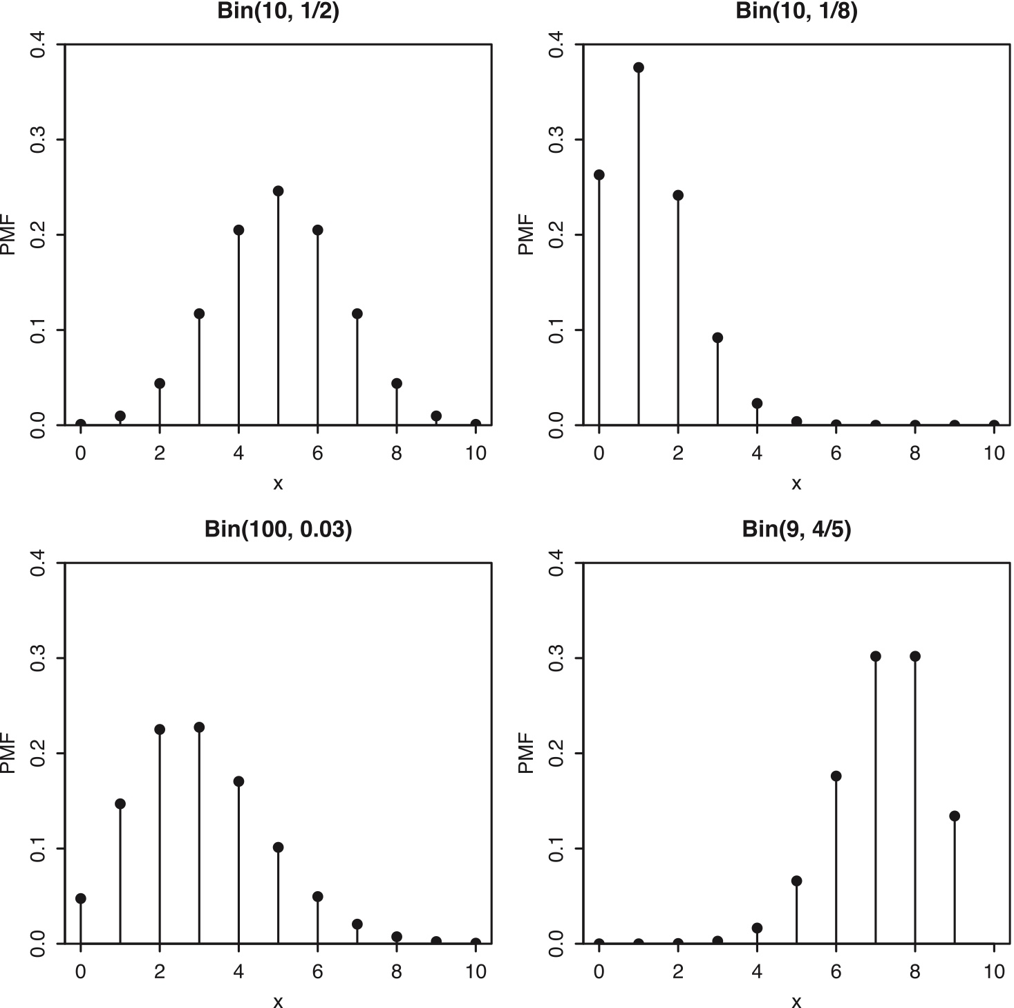
Figure 3.6: Some Binomial PMFs with different \(n\) and \(p\).
Theorem 3.3.7.
Let \(X\sim\mbox{Bin}(n,p)\), and \(q=1-p\) (we often use \(q\) to denote the failure probability of a Bernoulli trial). The \(n-X\sim\mbox{Bin}(n,q)\).
Corollary 3.3.8.
Let \(X\sim\mbox{Bin}(n,p)\) with \(p=1/2\) and \(n\) even.Then the distribution of \(X\) is symmetric about \(n/2\) in the sense that \(P(X=n/2+j)=P(X=n/2-j)\) for all nnonegative integers \(j\).
Example 3.3.9 (Coin tosses continued).
Going back to Example 3.1.2, we now know that \(X\sim\mbox{Bin}(2,1/2)\), \(Y\sim\mbox{Bin}(2,1/2)\), and \(I\sim\mbox{Bern}(1/2)\), where
- \(X\) is the number of Heads.
- \(Y\) is the number of Tails.
- \(I\) is the indicator of the first toss landing Heads.
3.7 Geometric distribution
Consider a sequence of independent Bernoulli trials, each with the same success probability \(p\in (0, 1)\), with trials performed until a success occurs.
Let \(X\) be the number of failures before the first successful trial. Then \(X\) has the Geometric distribution with parameter \(p\); we denote this by \(X\sim\mbox{Geom}(p)\).
For example, if we flip a fair coin until it lands Heads for the first time, then the number of Tails before the first occurrence of Heads is distributed as \(\mbox{Geom}(p)\).
To get the Geometric PMF from the story, imagine the Bernoulli trials as a string of 0’s (failures) ending in a single 1 (success). Each 0 has probability \(q=1-p\) and the final 1 has probability \(p\), so a string of \(k\) failures followed by one success has probability \(q^k p\), by multiplication rule.
Theorem 4.3.2 (Geometric PMF).
If \(X\sim\mbox{Geom}(p)\), then the PMF of \(X\) is \[ P (X=k)=q^k p \] for \(k=0,1,2,\ldots\), where \(q=1-p\).
- This is a valid PMF because
\[ \sum_{k=0}^\infty q^k p=p\sum_{k=0}^\infty q^k=p\cdot \frac{1}{(1-q)}=1. \]
There are differing conventions for the definition of the Geometric distribution; some sources define the Geometric as the total number of trials, including the success. In this book, the Geometric distribution excludes the success, and the First Success distribution includes the success.
Why this distribution is called Geometric distribution?
==Because the PMF is a geometric series==
3.8 Negative Binomial distribution
In a sequence of independent Bernoulli trials with success probability \(p\), if \(X\) is the number of failures before the \(r\)th success, then \(X\) is said to have the Negative Binomial distribution with parameters \(r\) and \(p\), denoted \(X\sim\mbox{NBin}(r, p)\).
- Both the Binomial and the Negative Binomial distributions are based on independent Bernoulli trials; they differ in the stopping rule and in what they are counting: the Binomial counts the number of successes in a fixed number of trials, while the Negative Binomial counts the number of failures until a fixed number of successes.
Theorem 4.3.8 (Negative Binomial PMF).
If \(X\sim\mbox{NBin(r,p)}\), then the PMF of \(X\) is \[ P(X=n)={n+r-1\choose r-1}p^r q^n \] for \(n=0,1,2,\ldots\), where \(q=1-p\).
3.9 Summary
Summarize distributions derived from a sequence of independent identical Bernoulli trials.
| Experiment | Random variable | Distribution |
|---|---|---|
| Run a Bernoulli trial independently for \(n\) times | The number of successes | Binomial(n, p) |
| Run a Bernoulli trial independently until witness the 1st success | The number of failures before the 1st success | Geometric(p) |
| Run a Bernoulli trial independently until witness \(r\) successes | The number of failures before \(r\)th success | Negative Binomial(r, p) |
3.10 Hypergeometric
If we have an urn filled with \(N\) balls, among which there are \(M\) white balls, and then we draw \(n\) balls out of the urn with replacement, the number of white balls we got has a \(\mbox{Bin}(n, M/N)\), since the draws are independent Bernoulli trials, each with probability \(p=M/N\) of success.
If we instead sample without replacement, then the number of white balls follows a Hypergeometric distribution.
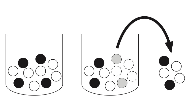
Story 3.4.1 (Hypergeometric distribution).
Consider an urn with \(N\) balls, among which there are \(M\) white balls, and then we draw \(n\) balls out of the urn without replacement.
Let \(X\) be the number of white balls in the sample. Then \(X\) is said to have the Hypergeometric distribution with parameters \(N\), \(K\) and \(n\); we denote this by \(X\sim\mbox{HGeom}(N,M,n)\), where
\(N\) = total population size
\(M\) = number of successes in the population
\(n\) = number of draws (sample size)
Theorem 3.4.2 (Hypergeometric PMF).
If \(X\sim\mbox{HGeom}(N,M,n)\), then the PMF of \(X\) is \[ P(X=k)=\frac{{M\choose k} {N-M\choose n-k}}{{N\choose n}}, \] for integers \(k\) satisfying \(0\leq k\leq M\) and \(0\leq n-k\leq N-M\), and \(P(X=k)=0\) otherwise.
\(k\) is the number of success in the sample.
Interpretation of PMF in the white ball, black ball setting:
We have \(\binom{N}{n}\) ways to draw \(n\) balls from \(N\) balls
Among those \(n\) sampled balls, there are \(k\) white balls and \(n-k\) black balls
Use multiplication rule, we can count the number of cases having \(k\) white balls is \[ \binom{M}{k}\binom{N-M}{n-k} \]
Typical application of hypergeometric distribution: “capture, label, and release”, a field sampling protocol used in ecology, zoology, or environmental monitoring.
Example 3.4.3 (Elk capture-recapture).
A forest has \(N\) elk.
Today, \(M\) of the elk are captured, tagged, and released into the wild. At a later date, \(n\) elk are recaptured at random. Assume that the recaptured elk are equally likely to be any set of \(n\) of the elk, e.g., an elk that has been captured does not learn how to avoid being captured again. By the story of the Hypergeometric, the number of tagged elk in the recaptured sample has the \(\mbox{HGeom}(N,M,n)\) distribution. The \(M\) tagged elk in this story correspond to the white balls and the \(N-M\) untagged elk correspond to the black balls. Instead of sampling \(n\) balls from the urn, we recapture \(n\) elk from the forest.
We have a population of \(N\) elks. After capture, tagged and released, those N elks can be categorized into two groups: tagged ones and untagged ones.
We recapture \(n\) elks. \(X\) is the number of tagged ones among the \(n\) recaptured elks.
“success”: the captured elk is tagged.
We can obtain \(\binom{N}{n}\) samples.
The event \(X=k\) means the recaptured sample is made of \(n\) tagged elks and \(n-k\) untagged elks. Thus, we have \[ \binom{M}{k} \binom{N-M}{n-k} \]
\[ P(\text{k tagged elks in the recaptured sample})=\frac{\binom{M}{k} \binom{N-M}{n-k}}{\binom{N}{n}} \]
In the textbook, Hyper geometric distribution is denoted as \(Hgeom(a, b, n)\) where \(a\) is the number of success in the population, and \(b\) is the number of failures in the population.
In this parameterization, \[ P(X=k)=\frac{\binom{a}{k}\binom{b}{n-k}}{\binom{a+b}{n}} \]
Theorem 3.4.5. The \(\mathrm{HGeom}(N, M, n)\) and \(\mathrm{HGeom}(N, n, M)\) distributions are identical. That is, if \(X \sim \mathrm{HGeom}(N, M, n)\) and \(Y \sim \mathrm{HGeom}(N, n, M)\), then \(X\) and \(Y\) have the same distribution.
\[ P(Y=y)=\frac{\binom{n}{y}\binom{N-n}{M-y}}{\binom{N}{M}} \]
Binomial vs. Hypergeometric
| Distribution | Sampling Type | Description |
|---|---|---|
| Binomial | With replacement (or independent trials) | Each trial is independent, and the probability of success stays constant. |
| Hypergeometric | Without replacement | Each draw affects the next one — the probability of success changes after each draw. |
The hypergeometric distribution approaches the binomial distribution when the population size \(N\) is much larger than the sample size \(n\).
Formally:
\[ n \ll N \]
or equivalently, when the sampling fraction
\[ \frac{n}{N} \]
is small (say, less than 5%).
In this case, removing a few items hardly changes the probabilities — so sampling without replacement behaves almost like sampling with replacement.
3.11 Discrete Uniform
Story 3.5.1 (Discrete Uniform distribution).
Let \(C\) be a finite, nonempty set of numbers. Choose one of these numbers uniformly at random (i.e., all values in \(C\) are equally likely). Call the chosen number \(X\). Then \(X\) is said to have the Discrete Uniform distribution with parameter \(C\); we denote this by \(X\sim\mbox{DUnif}(C)\).
The PMF of \(X\sim\mbox{DUnif(C)}\) is \[ P(X=x)=\frac{1}{|C|} \] for \(x\in C\) (and 0 otherwise).
PMF of a uniform distribution stays constant in the whole support.
For \(X\sim\mbox{DUnif}(C)\) and any \(A\subseteq C\), \[ P(X\in A)=\frac{|A|}{|C|}. \]
Generic example of discrete Uniform distribution:
| X | 0 | 1 | 2 |
|---|---|---|---|
| \(p_X\) | 1/3 | 1/3 | 1/3 |
Example 3.5.2 (Random slips of paper).
There are \(100\) slips of paper in a hat, each of which has one of the numbers \(1, 2,\ldots,100\) written on it, with no number appearing more than once. Five of the slips are drawn, one at a time.
First consider random sampling with replacement (with equal probabilities).
- What is the distribution of how many of the drawn slips have a value of at least 80 written on them?
==Step1: Define r.v. \(X\) as the number of drawn splips having at least 80 written on it.==
==Step2: Find the support, \(x=0, 1,2,3,4,5\)==
Success: the number of the drawn paper is equal to greater than 80
The number of Bernoulli trials \(n\)=5
The rate of success \(p=\frac{21}{100}\)
This is \(Binom(5, 0.21)\).
- What is the distribution of the value of the \(j\)th draw (for \(1 \leq j \leq 5\))?
Define r.v. \(Y\) as the value of \(j\)th draw
The support is \(y=1, 2, \ldots, 100\)
Since each draw is an independent and identical Bernoulli trial, without loss of generality, we can assume \(j=1\).
| Y | 1 | 2 | \(\ldots\) | 100 |
|---|---|---|---|---|
| \(p_Y\) | 1/100 | 1/100 | … | 1/100 |
- What is the probability that the number 100 is drawn at least once?
\[ P(\text{100 is drawn at least once})=1-P(\text{none of the draws has 100 on it})=1-(99/100)^5 \]
Now consider random sampling without replacement (with all sets of five slips equally likely to be chosen).
- What is the distribution of how many of the drawn slips have a value of at least 80 written on them?
HyperGeometric(N=100, M=21, n=5)
In the textbook, HyperGeometric distribution may be written as \(HGeom(21, 79, 5)\).
- What is the distribution of the value of the jth draw (for \(1\leq j\leq 5\))?
It is asking about the unconditional distribution of the value of \(j\)th draw.
By “unconditional”, it means “unconditioned on the results of 1st - (j-1)th draws”.
In other words, when the \(j\)th draw is performed, the values of previous draws are unknown.
This is still a discrete Uniform.
| Y | 1 | 2 | \(\ldots\) | 100 |
|---|---|---|---|---|
| \(p_Y\) | 1/100 | 1/100 | … | 1/100 |
- What is the probability that the number 100 is drawn at least once?
Recall: the sampling is without replacement, so 100 can only be drawn once. \[ \begin{split} P(\text{100 is drawn at least once})\\ &=P(\text{1st draw has 100 on it})+P(\text{2nd draw has 100 on it})+\cdots \\ &+P(\text{5th draw has 100 on it}) \end{split} \]
3.12 Cumulative distribution function (CDF)
Definition 3.6.1.
The cumulative distribution function (CDF) of an r.v. \(X\) is the function \(F_X\) given by \[ F_X (x) = P (X\leq x). \]
For discrete random variable \(X\) with support \(x_1, \ldots, x_n\), \[ p_X(x_j)=F_X(x_j)-F_X(x_{j-1}) \]
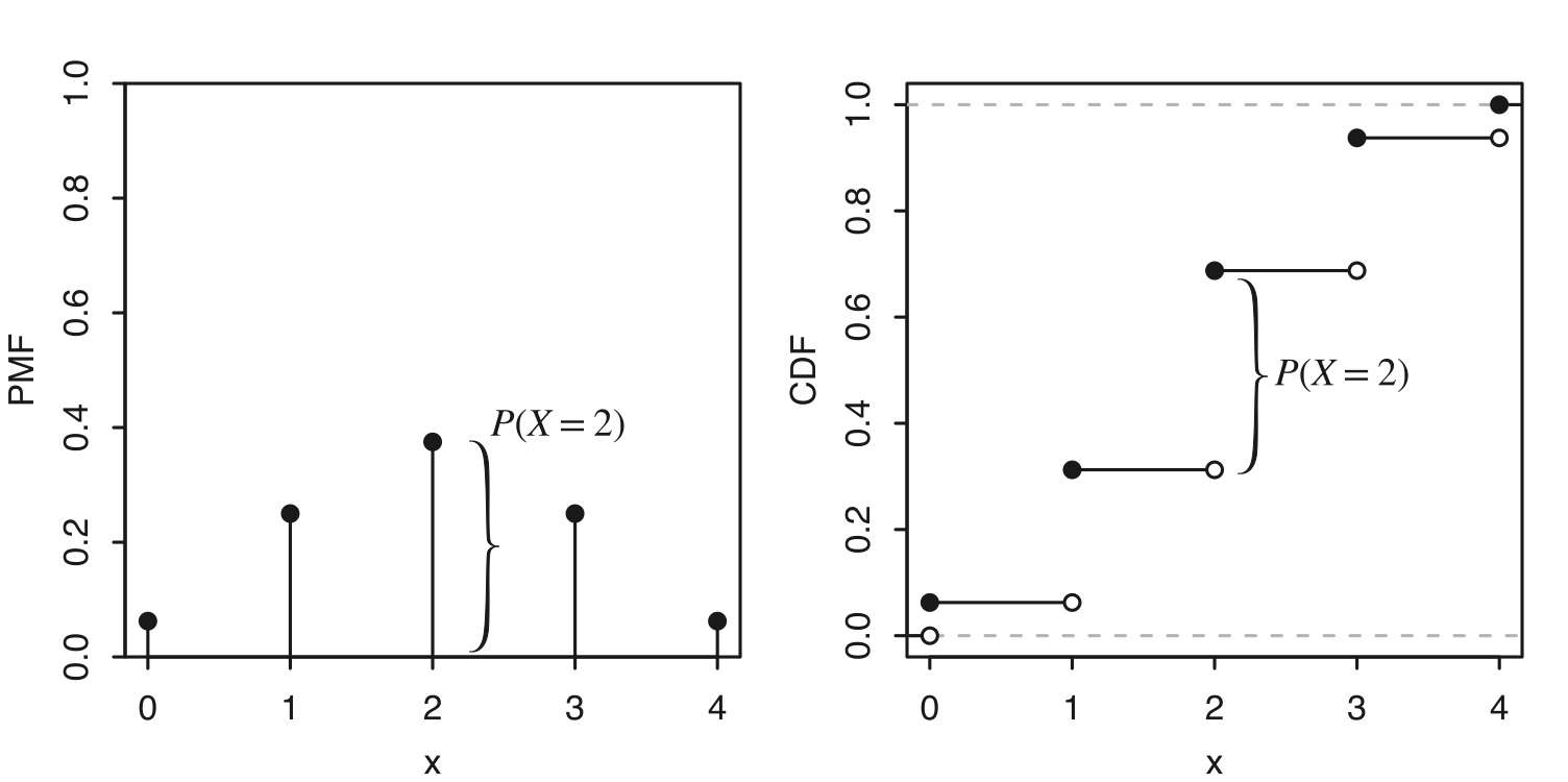
Example 3.6.2.
Let \(X\sim\mbox{Bin}(4,1/2)\).
\(P(X=x)={4\choose x} \Bigl(\frac{1}{2}\Bigr)^4\), \(x=0,1,2,3,4\).
\(P(X\leq 1.5)=P(X=0)+P(X=1)=\Bigl(\frac{1}{2}\Bigr)^4+4\Bigl(\frac{1}{2}\Bigr)^4=\frac{5}{16}\). We “accumulated” probilities of all possible values that are equal or less than 1.5
The CDF of a discrete r.v. is a piecewise function.
The CDF of a discrete r.v. consists of jumps and flat regions. The height of a jump in the CDF at \(x\) is equal to the value of the PMF at x.
The height of the jump in the CDF at 2 is the same as the height of the corresponding vertical bar in the PMF; this is indicated in the figure with curly braces.
Obtain CDF from PMF:
Step 1: list all values of \(x\) in the support of \(p_X\). In this example, the support contain \(0, 1, 2, 3, 4\)
| x | PMF | Simplified Value |
|---|---|---|
| 0 | \(p_X(1) = \binom{4}{0}\left(\frac{1}{2}\right)^0\left(\frac{1}{2}\right)^4 = \frac{1}{16}\) | 0.0625 |
| 1 | \(p_X(1) = \binom{4}{1}\left(\frac{1}{2}\right)^1\left(\frac{1}{2}\right)^3 = \frac{4}{16}\) | 0.25 |
| 2 | \(p_X(1) = \binom{4}{2}\left(\frac{1}{2}\right)^2\left(\frac{1}{2}\right)^2 = \frac{6}{16}\) | 0.375 |
| 3 | \(p_X(3) = \binom{4}{3}\left(\frac{1}{2}\right)^3\left(\frac{1}{2}\right)^1 = \frac{4}{16}\) | 0.25 |
| 4 | \(p_X(4) = \binom{4}{4}\left(\frac{1}{2}\right)^4\left(\frac{1}{2}\right)^0 = \frac{1}{16}\) | 0.0625 |
==Step 2: Create intervals on the domain of CDF using listed values in Step1 as breaking points==
Step 3: evaluate CDF by adding the values of PMF
| Intervals | \(F_X(x)\) |
|---|---|
| \((-\infty, 0)\) | 0 |
| [0, 1) | \(p_X(0)\), which accumulates probabilities to \(0\) |
| [1, 2) | \(p_X(0)+p_X(1)=F_X(0)+p_X(1)\), which accumulates probability to \(1\) |
| [2, 3) | \(p_X(0)+p_X(1)+p_X(2)=F_X(1)+p_X(2)\), which accumulates probability to \(2\) |
| [3, 4) | \(p_X(0)+p_X(1)+p_X(2)+p_X(3)=F_X(2)+p_X(3)\), which accumulates probability to \(3\) |
| \([4, \infty)\) | \(p_X(0)+p_X(1)+p_X(2)+p_X(3)+p_X(4)=F_X(3)+p_X(4)=1\), which accumulates probability to \(4\) |
Obtain PMF from CDF
| x | \(p_X(x)\) |
|---|---|
| 0 | \(F_X(0)-0\) |
| 1 | \(F_X(1)-F_X(0)\) |
| 2 | \(F_X(2)-F_X(1)\) |
| 3 | \(F_X(3)-F_X(2)\) |
| 4 | \(F_X(4)-F_X(3)\) |
\[ p_X(x_j)=F_X(x_j)-F_X(x_{j-1}) \]
where \(x_1, \ldots, x_n\) are points in the support.
Theorem 3.6.3 (Valid CDFs).
Any CDF \(F\) has the following properties.
- Non-decreasing: If \(x_1 < x_2\), then \(F(x_1)\leq F(x_2)\).
- Right-continuous: the CDF is continuous except possibly for having some jumps. Wherever there is a jump, the CDF is continuous from the right. That is, for any \(a\), we have \[ F(a)=\lim_{x\rightarrow a^+} F(x). \]
- Convergence to 0 and 1 in the limits: \[ \lim_{x\rightarrow -\infty}F(x)=0 \;\; \mbox{and} \;\; \lim_{x\rightarrow \infty}F(x)=1. \]
Proof.
We will only prove it for the case where \(F\) is the CDF of a discrete r.v. \(X\) whose possible values are \(0, 1, 2,\ldots\).
The first criterion is true since the event \(\{X \leq x_1\}\) is a subset of the event \(\{X \leq x_2\}\), so \(P(X\leq x_1) \leq P(X\leq x_2)\) (this does not depend on \(X\) being discrete).
For the second criterion, note that \[ P(X\leq x)=P(X\leq \lfloor x\rfloor), \] where \(\lfloor x\rfloor\) is the greatest integer less than or equal to \(x\). So \(F(a + b)=F(a)\) for any \(b>0\) that is small enough so that \(a+b<\lfloor a\rfloor+1\), e.g., for \(a=4.9\), this holds for \(0<b<0.1\). This implies \(F(a)=\lim_{x\rightarrow a^+} F(x)\).
For the third criterion, we have \(F(x)=0\) for \(x<0\), and
\[ \begin{split} \lim_{x\rightarrow \infty}F(x) & = \lim_{x\rightarrow \infty} P(X\leq \lfloor x\rfloor) \\ & = \lim_{x\rightarrow \infty}\sum_{n=0}^{\lfloor x\rfloor}P(X=n) \\ & = \sum_{n=0}^\infty P(X=n)=1. \end{split} \]
3.13 Functions of random variables
For example, imagine that two basketball teams (A and B) are playing a seven game match, and let \(X\) be the number of wins for team A (so \(X\sim\mbox{Bin}(7, 1/2)\) if the teams are evenly matched and the games are independent).
Then \(g(x)=7-x\) is the number of wins of and team B, and \[ h(x) = \left\{ \begin{array}{ll} 1 & \mbox{if}\;\; x\geq 4\\ 0 & \mbox{if}\;\; x<4. \end{array} \right. \] is the indicator of team A winning the majority of the games.
Since \(X\) is a random variable, both \(g(X)\) and \(h(X)\) are also random variables.
You may interpret \(g(X)\) as a composite function: \[ g(X(outcome))=g \circ X(outcome) \]
Definition 3.7.1 (Function of an r.v.).
For an experiment with sample space \(S\), an r.v. \(X\), and a function \(g : \mathbb{R}\rightarrow\mathbb{R}\), \(g(X)\) is the r.v. that maps \(s\) to \(g(X(s))\) for all \(s\in S\).
\(g(X)=\sqrt{X}\):
When \(g(x)\) is one to one mapping, it is easy to obtain the PMF of \(Y=g(X)\) directly from the PMF of \(X\):
| \(x\) | \(P(X=x)\) | \(y=g(x)\) | \(P(Y=y)\) |
|---|---|---|---|
| \(x_1\) | \(p_1\) | \(g(x_1)\) | \(p_1\) |
| \(x_2\) | \(p_2\) | \(g(x_2)\) | \(p_2\) |
| \(x_3\) | \(p_3\) | \(g(x_3)\) | \(p_3\) |
| \(\vdots\) | \(\vdots\) | \(\vdots\) | \(\vdots\) |
Example 3.7.2 (Random walk). obtain PMF of a function of r.v.
A particle moves \(n\) steps on a number line. The particle starts at 0, and at each step it moves 1 unit to the right or to the left, with equal probabilities. Assume all steps are independent.
Let \(Y\) be the particle’s position after \(n\) steps. Find the PMF of \(Y\).
Left: failure
Right: success
The number of trials: \(n\)
Let \(X\) be the number of success, then \(X\sim Bin(n, 1/2)\) \[ Y=X-(n-X)=2X-n \]
\[ P(Y=y)=P(2X-n=y)=P(X=\frac{y+n}{2})=\binom{n}{\frac{y+n}{2}}(0.5)^{\frac{y+n}{2}}(0.5)^{n-\frac{y+n}{2}}=\binom{n}{\frac{y+n}{2}}(0.5)^n \]
\[ y=-n,\ldots,n \]
Theorem 3.7.3 (PMF of \(g(X)\)).
Let \(X\) be a discrete r.v. and \(g : \mathbb{R}\rightarrow \mathbb{R}\). Then the support of \(g(X)\) is the set of all \(y\) such that \(g(x) = y\) for at least one \(x\) in the support of \(X\), and the PMF of \(g(X)\) is \[ P(g(X)=y)=\sum_{x: g(x)=y}P(X=x) \]
for all \(y\) in the support of \(g(X)\).
The support of \(Y=g(X)\) is the range of \(g(x)\) in the support of \(X\)
For example, if we have a r.v. \(X\) with support \((-\infty, \infty)\), and a function \(g(x)=|x|\).
What is the support of the new r.v. \(Y=g(X)\)?
The support of \(Y\) is \((0, \infty)\).
Example 3.7.4.
Continuing as in the previous example, let \(D\) be the particle’s distance from the origin after \(n\) steps. Assume that \(n\) is even. Find the PMF of \(D\).
\[ D=|Y| \]
\[ P(D=d)=P(|Y|=d)=P(Y=-d \mbox{ or } Y=d)=\binom{n}{\frac{-d+n}{2}}(0.5)^n+\binom{n}{\frac{d+n}{2}}(0.5)^n=2\binom{n}{\frac{d+n}{2}}(0.5)^n \]
\[ d=0, \ldots, n \] Definition 3.7.5 (Function of two r.v.s).
Given an experiment with sample space \(S\), if \(X\) and \(Y\) are r.v.s that map \(s\in S\) to \(X(s)\) and \(Y(s)\) respectively, then \(g(X, Y)\) is the r.v. that maps \(s\) to \(g(X(s), Y (s))\).
Example 3.7.6 (Maximum of two die rolls).
We roll two fair 6-sided dice. Let \(X\) be the number on the first die and \(Y\) the number on the second die. The following table gives the values of \(X\), \(Y\) , and \(\max(X, Y)\) under 7 of the 36 outcomes in the sample space, analogously to the table in Example 3.2.5.
Sample space:
| Y=1 | Y=2 | Y=3 | Y=4 | Y=5 | Y=6 | |
|---|---|---|---|---|---|---|
| X=1 | (1, 1) | (1, 2) | (1, 3) | (1, 4) | (1, 5) | (1, 6) |
| X=2 | (2, 1) | (2, 2) | (2, 3) | (2, 4) | (2, 5) | (2, 6) |
| X=3 | (3, 1) | (3, 2) | (3, 3) | (3, 4) | (3, 5) | (3, 6) |
| X=4 | (4, 1) | (4, 2) | (4, 3) | (4, 4) | (4, 5) | (4, 6) |
| X=5 | (5, 1) | (5, 2) | (5, 3) | (5, 4) | (5, 5) | (5, 6) |
| X=6 | (6, 1) | (6, 2) | (6, 3) | (6, 4) | (6, 5) | (6, 6) |
Joint PMF of X and Y: \[ p_{XY}(i, j)=P(X=i, Y=j)=\frac{1}{36}, \quad i,j=1,\ldots, 6 \]
Tabular form:
| \(p_{XY}(i, j)\) | Y=1 | Y=2 | Y=3 | Y=4 | Y=5 | Y=6 |
|---|---|---|---|---|---|---|
| X=1 | 1/36 | 1/36 | 1/36 | 1/36 | 1/36 | 1/36 |
| X=2 | 1/36 | 1/36 | 1/36 | 1/36 | 1/36 | 1/36 |
| X=3 | 1/36 | 1/36 | 1/36 | 1/36 | 1/36 | 1/36 |
| X=4 | 1/36 | 1/36 | 1/36 | 1/36 | 1/36 | 1/36 |
| X=5 | 1/36 | 1/36 | 1/36 | 1/36 | 1/36 | 1/36 |
| X=6 | 1/36 | 1/36 | 1/36 | 1/36 | 1/36 | 1/36 |
==Marginal PMF== of X and Y:
| \(p_{XY}(i, j)\) | Y=1 | Y=2 | Y=3 | Y=4 | Y=5 | Y=6 | \(p_X(i)\) |
|---|---|---|---|---|---|---|---|
| X=1 | 1/36 | 1/36 | 1/36 | 1/36 | 1/36 | 1/36 | 1/6 |
| X=2 | 1/36 | 1/36 | 1/36 | 1/36 | 1/36 | 1/36 | 1/6 |
| X=3 | 1/36 | 1/36 | 1/36 | 1/36 | 1/36 | 1/36 | 1/6 |
| X=4 | 1/36 | 1/36 | 1/36 | 1/36 | 1/36 | 1/36 | 1/6 |
| X=5 | 1/36 | 1/36 | 1/36 | 1/36 | 1/36 | 1/36 | 1/6 |
| X=6 | 1/36 | 1/36 | 1/36 | 1/36 | 1/36 | 1/36 | 1/6 |
| \(p_Y(j)\) | 1/6 | 1/6 | 1/6 | 1/6 | 1/6 | 1/6 |
Function of random variables \(Z=\max(X, Y)\):
| Max(X, Y) | Y = 1 | Y = 2 | Y = 3 | Y = 4 | Y = 5 | Y = 6 |
|---|---|---|---|---|---|---|
| X = 1 | 1 | 2 | 3 | 4 | 5 | 6 |
| X = 2 | 2 | 2 | 3 | 4 | 5 | 6 |
| X = 3 | 3 | 3 | 3 | 4 | 5 | 6 |
| X = 4 | 4 | 4 | 4 | 4 | 5 | 6 |
| X = 5 | 5 | 5 | 5 | 5 | 5 | 6 |
| X = 6 | 6 | 6 | 6 | 6 | 6 | 6 |
PMF of \(Z\): \[ \begin{split} P(Z=1) & = 1/36, \\ P(Z=2) & = 3/36, \\ P(Z=3) & = 5/36, \\ P(Z=4) & = 7/36, \\ P(Z=5) & = 9/36, \\ P(Z=6) & = 11/36. \end{split} \]
3.14 Independence of random variables
Definition 3.8.1 (Independence of two r.v.s).
Random variables \(X\) and \(Y\) are said to be independent if \[ P(X\leq x, Y\leq y)=P(X\leq x)P(Y\leq y), \] for all \(x,y\in \mathbb{R}\).
In the discrete case, this is equivalent to the condition \[ P(X=x, Y=y)=P(X=x)P(Y=y), \] for all \(x,y\) with \(x\) in the support of \(X\) and \(y\) in the support of \(Y\).
Definition 3.8.2 (Independence of many r.v.s).
Random variables \(X_1,\ldots,X_n\) are independent if \[ P(X_1\leq x_1,\ldots,X_n\leq x_n)=P(X_1\leq x_1)\ldots P(X_n\leq x_n), \] for all \(x_1,\ldots,x_n\in\mathbb{R}\).
- For infinitely many r.v.s, we say that they are independent if every finite subset of the r.v.s is independent.
- If we can find even a single list of values \(x_1,\ldots,x_n\) for which the above equality fails to hold, then \(X_1,\ldots,X_n\) are not independent.
If \(X_1,\ldots,X_n\) are independent, then they are pairwise independent, i.e., \(X_i\) is independent of \(X_j\) for \(i\ne j\).
- Pairwise independence does not imply independence in general
Example 3.8.4. In a roll of two fair dice, if \(X\) is the number on the first die and \(Y\) is the number on the second die, then \(X + Y\) is not independent of \(X - Y\).
Image extreme cases, such as \(X+Y=12\).
If \(X\) and \(Y\) are independent then it is also true, for example, that \(X^2\) is independent of \(Y^3\), since if \(X^2\) provided information about \(Y^3\) then \(X\) would give information about \(Y\).
In general, if \(X\) and \(Y\) are independent then any function of \(X\) is independent of any function of \(Y\).
Theorem 3.8.5 (Functions of independent r.v.s).
If \(X\) and \(Y\) are independent r.v.s, then any function of \(X\) is independent of any function of \(Y\).
Definition 3.8.6 (i.i.d.).
We will often work with random variables that are independent and have the same distribution. We call such r.v.s independent and identically distributed, or i.i.d. for short.
“Independent” and “identically distributed” are two often confused but completely different concepts. Random variables are independent if they provide no information about each other; they are identically distributed if they have the same PMF (or equivalently, the same CDF).
Whether two r.v.s are independent has nothing to do with whether or not they have the same distribution. We can have r.v.s that are:
Independent and identically distributed: Let \(X\) be the result of a die roll, and let \(Y\) be the result of a second, independent die roll. Then \(X\) and \(Y\) are i.i.d.
Independent and not identically distributed: Let \(X\) be the result of a die roll, and let \(Y\) be the closing price of the Dow Jones (a stock market index) a month from now. Then \(X\) and \(Y\) provide no information about each other (one would fervently hope), and \(X\) and \(Y\) do not have the same distribution.
Dependent and identically distributed: Let \(X\) be the number of Heads in \(n\) independent fair coin tosses, and let \(Y\) be the number of Tails in those same \(n\) tosses. Then \(X\) and \(Y\) are both distributed \(\mbox{Bin}(n, 1/2)\), but they are highly dependent: if we know \(X\), then we know \(Y\) perfectly.
Dependent and not identically distributed: Let \(X\) be the indicator of whether the majority party retains control of the House of Representatives in the U.S. after the next election, and let \(Y\) be the average favorability rating of the majority party in polls taken within a month of the election. Then \(X\) and \(Y\) are dependent, and \(X\) and \(Y\) do not have the same distribution.
Theorem 3.8.8.
If \(X\sim \mbox{Bin}(n, p)\), viewed as the number of successes in \(n\) independent Bernoulli trials with success probability \(p\), then we can write \(X=X_1+\ldots + X_n\) where the \(X_i\) are i.i.d. \(\mbox{Bern}(p)\).
Theorem 3.8.9.
If \(X\sim\mbox{Bin}(n,p)\), \(Y\sim\mbox{Bin}(m,p)\), and \(X\) is independent of \(Y\) , then \(X + Y\sim\mbox{Bin}(n + m, p)\).
Definition 3.8.10 (Conditional independence of r.v.s).
Random variables \(X\) and \(Y\) are conditionally independent given an r.v. \(Z\) if for all \(x,y\in\mathbb{R}\) and all \(z\) in the support of \(Z\) \[ P(X\leq x, Y\leq y\mid Z=z)=P(X\leq x\mid Z=z) P(Y\leq y\mid Z=z). \] For discrete r.v.s, an equivalent definition is to require \[ P(X=x, Y=y\mid Z=z)=P(X=x\mid Z=z) P(Y=y\mid Z=z). \]
Definition 3.8.11 (Conditional PMF).
For any discrete r.v.s \(X\) and \(Z\), the function \(P (X = x\mid Z = z)\), when considered as a function of \(x\) for fixed \(z\), is called the conditional PMF of \(X\) given \(Z = z\).
- Independence of r.v.s does not imply conditional independence, nor vice versa.
Example 3.8.12 (Matching pennies).
Consider the simple game called matching pennies. Each of two players, A and B, has a fair penny. They flip their pennies independently. If the pennies match, A wins; otherwise, B wins. Let \(X\) be 1 if A’s penny lands Heads and \(-1\) otherwise, and define \(Y\) similarly for B (the r.v.s \(X\) and \(Y\) are called random signs).
Let \(Z=XY\).
Example 3.8.13 (Two friends).
Consider again the “I have only two friends who ever call me” scenario from Example 2.5.11, except now with r.v. notation.
Let \(X\) be the indicator of Alice calling me next Friday,
\(Y\) be the indicator of Bob calling me next Friday, and
\(Z\) be the indicator of exactly one of them calling me next Friday. Then \(X\) and \(Y\) are independent (by assumption). But given \(Z=1\), we have that \(X\) and \(Y\) are completely dependent: given that \(Z=1\), we have \(Y=1-X\).
Example 3.8.14 (Mystery opponent).
Suppose that you are going to play two games of tennis against one of two identical twins. Against one of the twins, you are evenly matched, and against the other you have a \(3/4\) chance of winning. Suppose that you can’t tell which twin you are playing against until after the two games.
Let \(Z\) be the indicator of playing against the twin with whom you’re evenly matched, and let \(X\) and \(Y\) be the indicators of victory in the first and second games, respectively.
3.15 Connections between Binomial and Hypergeometric
The Binomial and Hypergeometric distributions are connected in two important ways. As we will see in this section, we can get from the Binomial to the Hypergeometric by conditioning, and we can get from the Hypergeometric to the Binomial by taking a limit of the population size.
Example 3.9.1 (Fisher exact test).
A scientist wishes to study whether women or men are more likely to have a certain disease, or whether they are equally likely. A random sample of \(n\) women and \(m\) men is gathered, and each person is tested for the disease (assume for this problem that the test is completely accurate).
The numbers of women and men in the sample who have the disease are \(X\) and \(Y\) respectively, with \(X\sim \mbox{Bin}(n, p_1)\) and \(Y\sim\mbox{Bin}(m, p_2)\), independently.
Here \(p_1\) and \(p_2\) are unknown, and we are interested in testing whether \(p_1=p_2=p\) (this is known as a null hypothesis in statistics).
| Women | Men | Total | |
|---|---|---|---|
| Disease | \(x\) | \(r-x\) | \(r\) |
| No disease | \(n-x\) | \(m-r+x\) | \(n+m-r\) |
| Total | \(n\) | \(m\) | \(n+m\) |
The Fisher exact test is based on conditioning on both the row and column sums, so \(n\), \(m\), \(r\) are all treated as fixed, and then seeing if the observed value of \(X\) is “extreme” compared to this conditional distribution.
Assuming the null hypothesis (\(p_1=p_2=p\)), find the conditional PMF of \(X\) given \(X+Y=r\).
\[ X\sim Bin(n, p)\\ Y\sim Bin(m, p) \]
\[ \begin{split} P(X=x\mid X+Y=r)&=\frac{P(X+Y=r\mid X=x)P(X=x)}{P(X+Y=r)} \\ &=\frac{P(Y=r-x)P(X=x)}{} \\ &=\frac{\binom{m}{r-x}p^{r-x}(1-p)^{m-r+x}\binom{n}{x}p^x(1-p)^{n-x}}{\binom{m+n}{r}p^r(1-p)^{m+n-r}} \\ &=\frac{\binom{m}{r-x}\binom{n}{x}}{\binom{m+n}{r}} \end{split} \] which is the PMF of \(HGeom(m+n, n ,r)\) or \(HGeom(n, m, r)\) (textbook parameterization).
In the elk story, we are interested in the distribution of the number of tagged elk in the recaptured sample. By analogy, think of women as tagged elk and men as untagged elk. Instead of recapturing r elk at random from the forest, we infect \(X + Y=r\) people with the disease; under the null hypothesis, the set of diseased people is equally likely to be any set of \(r\) people. Thus, conditional on \(X+Y=r\), \(X\) represents the number of women among the \(r\) diseased individuals. This is exactly analogous to the number of tagged elk in the recaptured sample, which is distributed \(\mbox{HGeom}(n, m, r)\).
An interesting fact, which turns out to be useful in statistics, is that the conditional distribution of \(X\) does not depend on \(p\): unconditionally, \(X\sim\mbox{Bin}(n,p)\), but \(p\) disappears from the parameters of the conditional distribution! This makes sense upon reflection, since once we know \(X+Y=r\), we can work directly with the fact that we have a population with \(r\) diseased and \(n+m-r\) undiseased people, without worrying about the value of \(p\) that originally generated the population. This motivating example serves as a proof of the following theorem.
Theorem 3.9.2.
If \(X\sim\mbox{Bin}(n,p)\), \(Y\sim\mbox{Bin}(m,p)\), and \(X\) is independent of \(Y\) , then the conditional distribution of \(X\) given \(X+Y=r\) is \(\mbox{HGeom}(n,m,r)\).
Theorem 3.9.3.
If \(X\sim\mbox{HGeom}(N,M,n)\) and \(N \rightarrow \infty\) such that \(p = M/N\) remains fixed, then the PMF of \(X\) converges to the \(\mbox{Bin}(n, p)\) PMF.
Proof:
Let’s use the more common parameterization of Hyper Geometric distribution, \(HGeom(N, M, n)\), where \(N\) is the population size, \(w\) is the number of success in the population and \(n\) is the sample size. \[ X\sim HGeom(N, M, n) \]
\[ p=\frac{M}{N} \]
By Theorem 3.4.5, \(HGeom(N, M, n)\) is the identical with \(HGeom(N, n, M)\).
\[ \begin{split} P(X=k) &= \frac{\binom{M}{k}\binom{N-M}{n-k}}{\binom{N}{n}}\\ &= \frac{\binom{n}{k}\binom{N-n}{M-k}}{\binom{N}{M}}\\ &=\binom{n}{k}\frac{(N-n)!}{(M-k)!(N-n-M+k)!}\frac{M!(N-M)!}{N!}\\ &=\binom{n}{k}\frac{(N-n)!}{N!}\frac{M!}{(M-k)!}\frac{(N-M)!}{(N-M-(n-k))!}\\ \\ &=\binom{n}{k}\frac{1}{N(N-1)\cdots(N-n+1)}\frac{M(M-1)\cdots(M-k+1)}{1}\frac{(N-M)(N-M-1)\cdots(N-M-(n-k)+1)}{1}\\ \\ &=\binom{n}{k}\frac{\left[M(M-1)\cdots(M-k+1)\right]\left[(N-M)(N-M-1)\cdots(N-M-(n-k)+1)\right]}{N(N-1)\cdots(N-n+1)}\\ \\ &=\binom{n}{k}\frac{\left[\frac{M}{N}(\frac{M}{N}-\frac{1}{N})\cdots(\frac{M}{N}-\frac{k-1}{N})\right]\left[\frac{(N-M)}{N}(\frac{(N-M)}{N}-\frac{1}{N})\cdots\frac{(N-M)}{N}-\frac{(n-k-1)}{N})\right]}{1(1-1/N)\cdots(1-(n-1)/N)} \\ \\ &=\binom{n}{k}\frac{[p(p-\frac{1}{N})\cdots(p-\frac{k-1}{N})][(1-p)((1-p)-\frac{1}{N})\cdots((1-p)-\frac{(n-k-1)}{N})]}{1\left(1-\frac{1}{N}\right)\cdots\left(1-\frac{n-1}{N}\right)} \end{split} \]
The stories of the Binomial and Hypergeometric provide intuition for this result: given an urn with \(M\) white balls and \(N-M\) black balls, the Binomial distribution arises from sampling \(n\) balls from the urn with replacement, while the Hypergeometric arises from sampling without replacement. As the number of balls in the urn grows very large relative to the number of balls that are drawn, sampling with replacement and sampling without replacement become essentially equivalent.
In practical terms, this theorem tells us that if \(N\) is large relative to \(n\), we can approximate the \(\mbox{HGeom}(N, M, n)\) PMF by the \(\mbox{Bin}(n,M/N)\) PMF.
3.15.1 Problem 14 — Poisson Purchases
Let \(X\) be the number of purchases that Fred will make on a certain online site during a fixed period. Suppose the PMF of \(X\) is \(P(X=k)=e^{-\lambda}\lambda^k/k!\) for \(k=0,1,2,\ldots\) (i.e., \(X\sim\text{Poisson}(\lambda)\)). \[ P(X=k)=\frac{e^{-\lambda}\lambda^k}{k!} \] (a) Find \(P(X\ge 1)\) and \(P(X\ge 2)\) without summing infinite series. \[ P(X\ge 1)=1-P(X=0)=1-e^{-\lambda} \\ P(X\ge 2)=1-P(X=0)-P(X=1) \] (b) Suppose the company only knows about people who have made at least one purchase (a user must set up an account to make a purchase; someone who has never purchased doesn’t appear in the database). The company then observes \(X\) from the conditional distribution given \(X\ge 1\). Find the conditional PMF of \(X\) given \(X\ge 1\) (this conditional distribution is called a truncated Poisson distribution).
\[ P(X=k \mid X \ge 1)=\frac{P(X=1, X\ge 1)}{P(X\ge 1)}=\frac{P(X=1)}{1-e^{-\lambda}}, \quad k=1, 2, \ldots \]
3.15.2 Problem 24
Let \(X\) be the number of Heads in \(10\) fair coin tosses.
- Find the conditional PMF of \(X\), given that the first two tosses both land Heads. \[ X=2,3\ldots, 10 \]
\[ P(X=2\mid \text{first two are Heads})=\frac{1}{2^8} \\ P(X=3\mid \text{first two are Heads})=\frac{\binom{8}{1}}{2^8} \\ P(X=4\mid \text{first two are Heads})=\frac{\binom{8}{2}}{2^8} \\ \cdots \]
\[ P(X=k\mid \text{first two are Heads})=\frac{\binom{8}{k-2}}{2^c},\quad k=2,3\ldots, 10 \]
- Find the conditional PMF of \(X\), given that at least two tosses land Heads \[ X=2,3\ldots, 10 \]
\[ P(\text{At least two tosses are Heads})=1-P(\text{no head})-P(\text{only one head}) =1-\frac{\binom{10}{1}}{2^{10}}-\frac{\binom{10}{2}}{2^{10}} \]
\[ P(X=2\mid \text{At least two tosses are Heads})=\frac{\binom{10}{2}}{2^{10}-\binom{10}{1}-\binom{10}{2}} \\ P(X=3\mid \text{At least two tosses are Heads})=\frac{\binom{10}{3}}{2^{10}-\binom{10}{1}-\binom{10}{2}} \\ \cdots \]
\[ P(X=k\mid \text{At least two tosses are Heads})=\frac{\binom{10}{k}}{2^{10}-\binom{10}{1}-\binom{10}{2}},\quad k=2,\ldots, 10 \]