Chapter 4 Item Fit

Let’s find out if the data fit the model. Use the tam.fit function to compute fit statistics, then display. We note that items V1 and V2 have outfits that are drastically different from the items’ infit values. We also note that infit values of V1 and V2 are different from any of the other items. We note that V1 is “over fitting,” it’s outfit and infit values being well below 1, while V2 is “underfitting.” This means that item V1 is too predictable - the amount of information is well predicted from other items which means it provides little new information above and beyond the other items. On the other hand, the underfitting V2 item has too much randomness.

To review, an item’s fit starts with its residuals.A residual is the observed response minus the expected response. The expected response is the probability of a student endorsing and item category or getting an item correct. The observed response is the student’s actual response. So, if a student is expected to get an item right with a probability of 40%, and the student gets the item right, then the residual is $1 - .40 = .60$.

To get outfit:

$$Z_{si}=\frac{X_{si}-E(X_{si})}{Var(X_{si})}$$

Where $X_{si}$ is the observed response of the s to item i. $E(X_{si})$ is the expected response of student s to item i. This is just the result of the Rasch model - the probability of getting an item correct or selecting an item category. $Var(X_{si})$ is simply $E(X_{si})(1-E(X_{si}))$.

Outfit of item i, is then:

$$Outfit_i = \frac{\sum_s Z_{si}^2}{n}$$

And, Infit, of item i is calculated:

$$Infit_i = \frac{\sum_s Z_{si}^2 W_{si}}{\sum_sW_{si}}$$

Note, that W are item specific weights coming from $Var(X_{si})$.

We don’t need to do this manually, and can instead use TAM.

However, outfit is “outlier” sensitive whereas “infit” is not. This implies that for V2 there might be a few responses that are particularly random/unexpected.

fit <- tam.fit(mod1)

## Item fit calculation based on 15 simulations
## |**********|
## |----------|

str(fit)

## List of 3
##  $ itemfit:'data.frame': 15 obs. of  9 variables:
##   ..$ parameter   : Factor w/ 15 levels "V1","V10","V11",..: 1 8 9 10 11 12 13 14 15 2 ...
##   ..$ Outfit      : num [1:15] 0.635 3.619 1.024 0.962 1.044 ...
##   ..$ Outfit_t    : num [1:15] -8.247 16.695 0.464 -0.677 1.198 ...
##   ..$ Outfit_p    : num [1:15] 1.62e-16 1.42e-62 6.43e-01 4.99e-01 2.31e-01 ...
##   ..$ Outfit_pholm: num [1:15] 2.27e-15 2.12e-61 1.00 1.00 1.00 ...
##   ..$ Infit       : num [1:15] 0.834 1.235 1.031 0.98 1.035 ...
##   ..$ Infit_t     : num [1:15] -3.437 2.305 0.604 -0.346 0.965 ...
##   ..$ Infit_p     : num [1:15] 0.000589 0.021159 0.545702 0.729449 0.334344 ...
##   ..$ Infit_pholm : num [1:15] 0.00884 0.29622 1 1 1 ...
##  $ time   : POSIXct[1:2], format: "2021-03-04 16:50:35" ...
##  $ CALL   : language tam.fit(tamobj = mod1)
##  - attr(*, "class")= chr "tam.fit"

View(fit$itemfit)

parameter	Outfit	Outfit_t	Outfit_p	Outfit_pholm	Infit	Infit_t	Infit_p	Infit_pholm
V1	0.6348193	-8.2470850	0.0000000	0	0.8340363	-3.4365960	0.0005891	0.0088361
V2	3.6191206	16.6953650	0.0000000	0	1.2351540	2.3051395	0.0211588	0.2962226
V3	1.0244030	0.4639721	0.6426677	1	1.0314371	0.6042125	0.5457024	1.0000000
V4	0.9622681	-0.6767866	0.4985413	1	0.9800337	-0.3458590	0.7294487	1.0000000
V5	1.0441221	1.1979991	0.2309174	1	1.0353141	0.9654005	0.3343443	1.0000000
V6	1.0008682	0.0221932	0.9822939	1	1.0025780	0.0904614	0.9279206	1.0000000
V7	0.9645949	-1.3434885	0.1791139	1	0.9769153	-0.8673938	0.3857263	1.0000000
V8	0.9740113	-1.0067846	0.3140383	1	0.9742177	-0.9916475	0.3213695	1.0000000
V9	0.9784955	-0.8048260	0.4209201	1	0.9819962	-0.6720271	0.5015665	1.0000000
V10	1.0126241	0.1624851	0.8709238	1	1.0023939	0.0535191	0.9573183	1.0000000
V11	0.9541706	-0.6728552	0.5010394	1	0.9950074	-0.0557559	0.9555363	1.0000000
V12	1.0421713	1.0261736	0.3048098	1	1.0151186	0.3826206	0.7020011	1.0000000
V13	0.8270982	-1.7376315	0.0822758	1	0.9918696	-0.0471409	0.9624009	1.0000000
V14	0.9615502	-1.3792037	0.1678320	1	0.9771779	-0.8110648	0.4173285	1.0000000
V15	0.9824680	-0.6776275	0.4980079	1	0.9821499	-0.6802111	0.4963708	1.0000000

4.0.1 Exercise:

1. Which items fit best? Which items fit worst?
2. How many, if any items, are outside the traditional bounds of mean-square item fit [.75, 1.33]?

4.1 Optional - Visualizing Item Fit

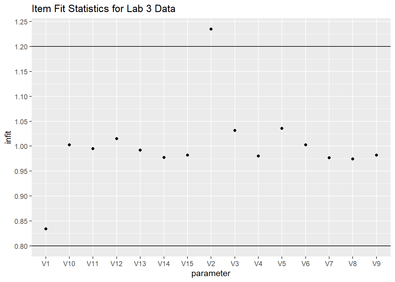
If you’d like, we can use default WrightMap functionality to plot item fit statistics. In the fit object, itemfit is a dataframe containing various fit statistics. We’ll plot infit with a lowerbound of .75 (in mean-square error units) and an upper bound of 1.33

The nice thing is that you can create unique fitbounds for each item (such that it’s sensitive to sample size). However, if we want all the same fit values, we have to just repeat the fit value (in our case, there are 15 items).

infit <- fit$itemfit$Infit

upper_bound <- rep(x = 1.33, times =15) # this repeats 1.33 fifteen times
lower_bound <- rep(x = .75, times = 15) 

# running fitgraph


fitgraph(fitEst = infit, fitLB = lower_bound, fitUB = upper_bound, itemLabels = names(hls))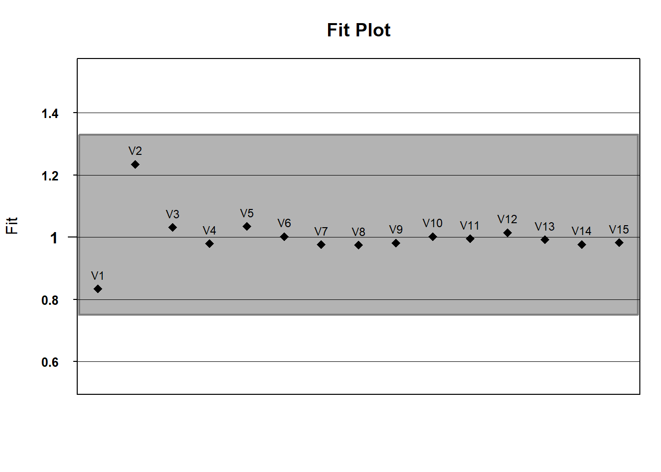

# what about outfit?
outfit <- fit$itemfit$Outfit


fitgraph(fitEst = outfit, fitLB = lower_bound, fitUB = upper_bound, itemLabels = names(hls))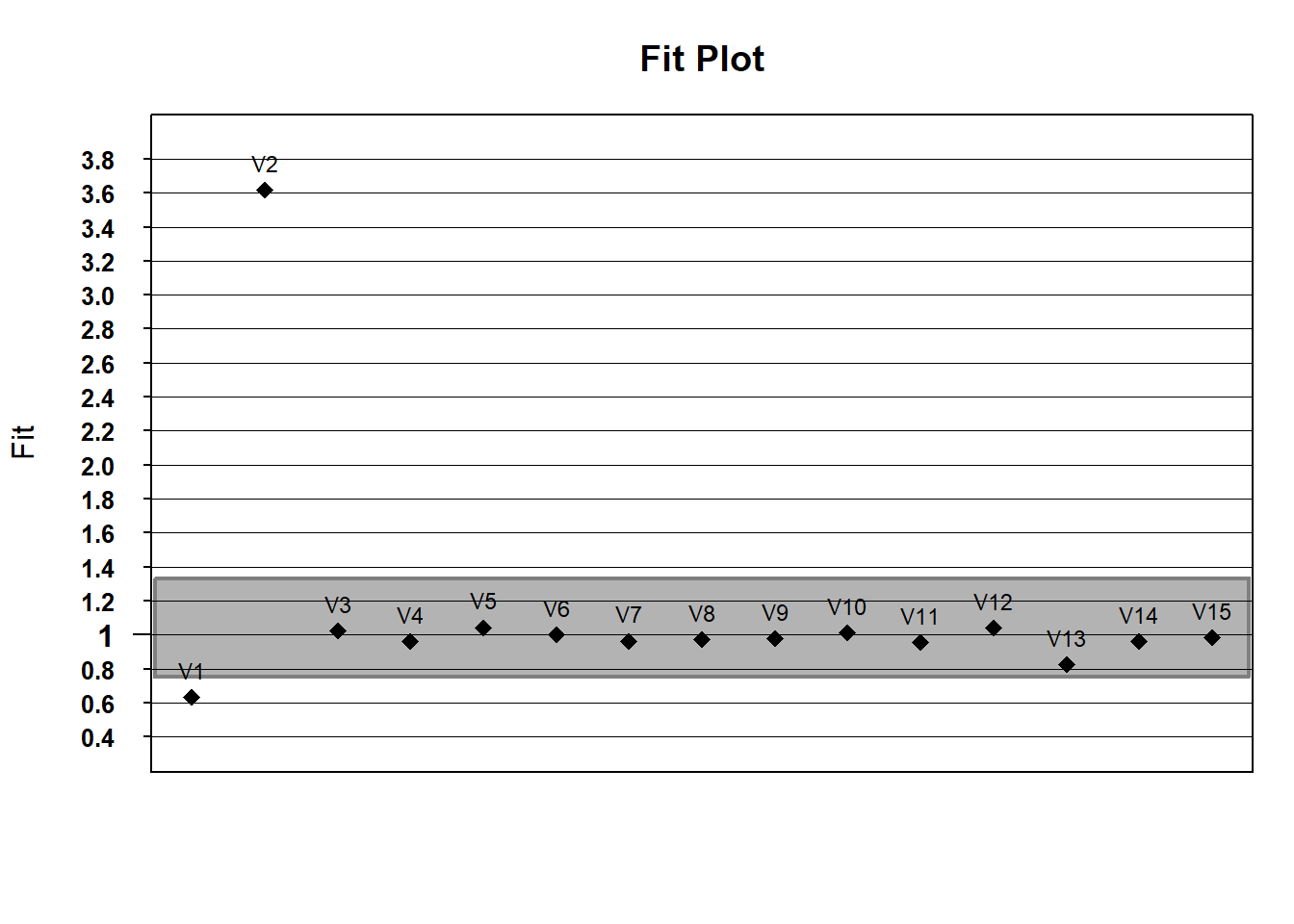

If you wanted to do this with ggplot - play with the code to try to change the fit limits or plot outfit instead of infit.

# put the fit data in a dataframe
fit_stats <- fit$itemfit

fit_stats %>%
  ggplot(aes(x=parameter, y = infit)) + 
  geom_point() + 
  geom_hline(yintercept = 1.2) +
  geom_hline(yintercept = .8) +
  scale_y_continuous(breaks = scales::pretty_breaks(n = 15)) + 
  ggtitle("Item Fit Statistics for Lab 3 Data")