Chapter 5 The Rasch Rating Scale Model
5.1 Introduction
This is the second part of lab 6. You do not need to watch lab6a to run this lab. However, if you are following along, you do not need to re-read in the data we’ll be using if it’s already in your environment. We tend to use the Partial Cedit Model (PCM) when the item categories, and hence thresholds, may not be the same across items. This allows for items with different response options (i.e., an item with two response options, and an item with three response options on the same assessment). The rating scale model (RSM), is an alternative model for this setup. In this formulation, the items have the same response options, and the thresholds, or \(\tau\)s (representing the deviance of the particular category from the overall item difficulty or severity) are the same across items. Therefore, items can have different overall item difficulties/severities.
Goals:
1. Learn how to run the rating scale model in TAM.
2. Learn how to interpret the rating scale model.
3. Learn how to do simple model comparison checking.
4. Bonus: Use the eRm package for improved person item maps.
The Rating Scale Model (RSM) can be expressed as follows.
\[P(X_{si} = x) = \frac{exp[\sum_{k=0}^x(\theta_s-\delta_{i}+\tau_{k})]}{\sum_{h=0}^{m_i}exp[\sum_{k=0}^h(\theta_s-\delta_{i} + \tau_{k})]}\].
Here, \(\delta_i\) is the overall item difficulty, and \(\tau_k\) is the particular threshold deviance for category \(k\). In the PCM, the \(\tau\) is item specific, it’s the “jump” of the category from the overall item difficulty. Note that i indexes item, and k indexes category. So, each \(\tau\) is the same for each item because it is not indexed by item.
library(tidyverse)
library(TAM)
library(eRm)
library(WrightMap)
5.2 Data
Data comes from a subset of the Health Literacy Survey.
These are the items in case you’re interested (it doesn’t matter, but here they are…)
On a scale from very easy to very difficult, how easy would you say it is to:
1. find information on treatments of illnesses that concern you?
2. find out where to get professional help when you are ill?
3. understand what your doctor says to you?
4. understand your doctor’s or pharmacist’s instruction on how to take a prescribed medicine?
5. judge when you may need to get a second opinion from another doctor?
6. use information the doctor gives you to make decisions about your illness?
7. follow instructions from your doctor or pharmacist?
8. find information on how to manage mental health problems like stress or depression?
9. understand health warnings about behavior such as smoking, low physical activity and drinking too much?
10. understand why you need health screenings?
11. judge if the information on health risks in the media is reliable?
12. decide how you can protect yourself from illness based on information in the media?
13. find out about activities that are good for your mental well-being?
14. understand advice on health from family members or friends?
15. understand information in the media on how to get healthier?
16. judge which everyday behavior is related to your health?
The Likert scale contains four response options (very easy, easy, difficult, very difficult).
5.2.1 Reading in the data
hls2 <- read_csv("https://raw.githubusercontent.com/danielbkatz/DBER_Rasch-data/master/data/hls_poly_scale.csv")5.2.2 Brief exploration of the data
apply(hls2, 2, table)## Hls1 Hls2 Hls3 Hls4 Hls5 Hls6 Hls7 Hls8 Hls9 Hls10 Hls11
## 0 63 76 129 160 65 90 140 50 146 139 47
## 1 204 207 176 148 166 196 162 154 144 163 116
## 2 44 32 11 7 78 26 12 101 21 13 130
## 3 6 2 1 2 8 5 3 12 6 2 24
## Hls12 Hls13 Hls14 Hls15 Hls16
## 0 44 52 64 52 69
## 1 138 176 181 148 185
## 2 119 83 60 105 57
## 3 16 6 12 12 65.3 Reviewing the Partial Credit Model
To have a model to compare, we’ll run a partial credit model in TAM. We won’t get too far into analyzing the data here, since we did that in the last lab. However as a reminder, we’ll run through the steps.
Remember - the partial credit model allows for the thresholds to differ for each item.
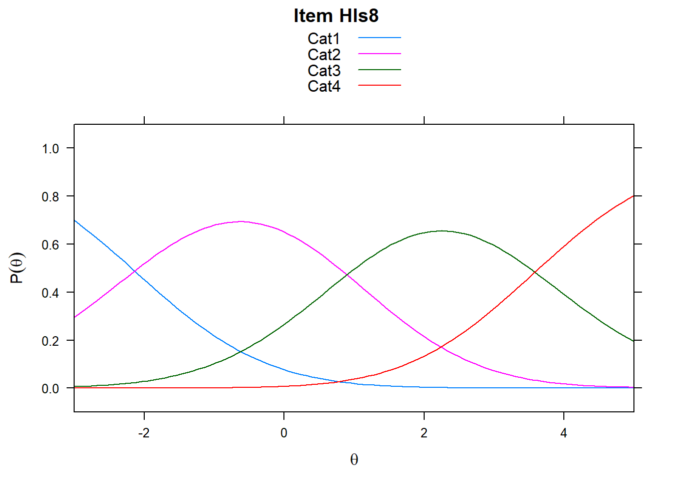
For clarity, look at Hls8 and Hls9. Which one is harder?
mod_pcm <- tam(hls2)5.3.1 Plot and look at difficulties/thresholds
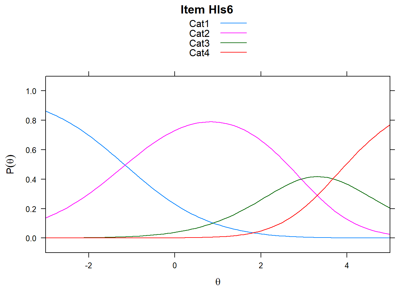
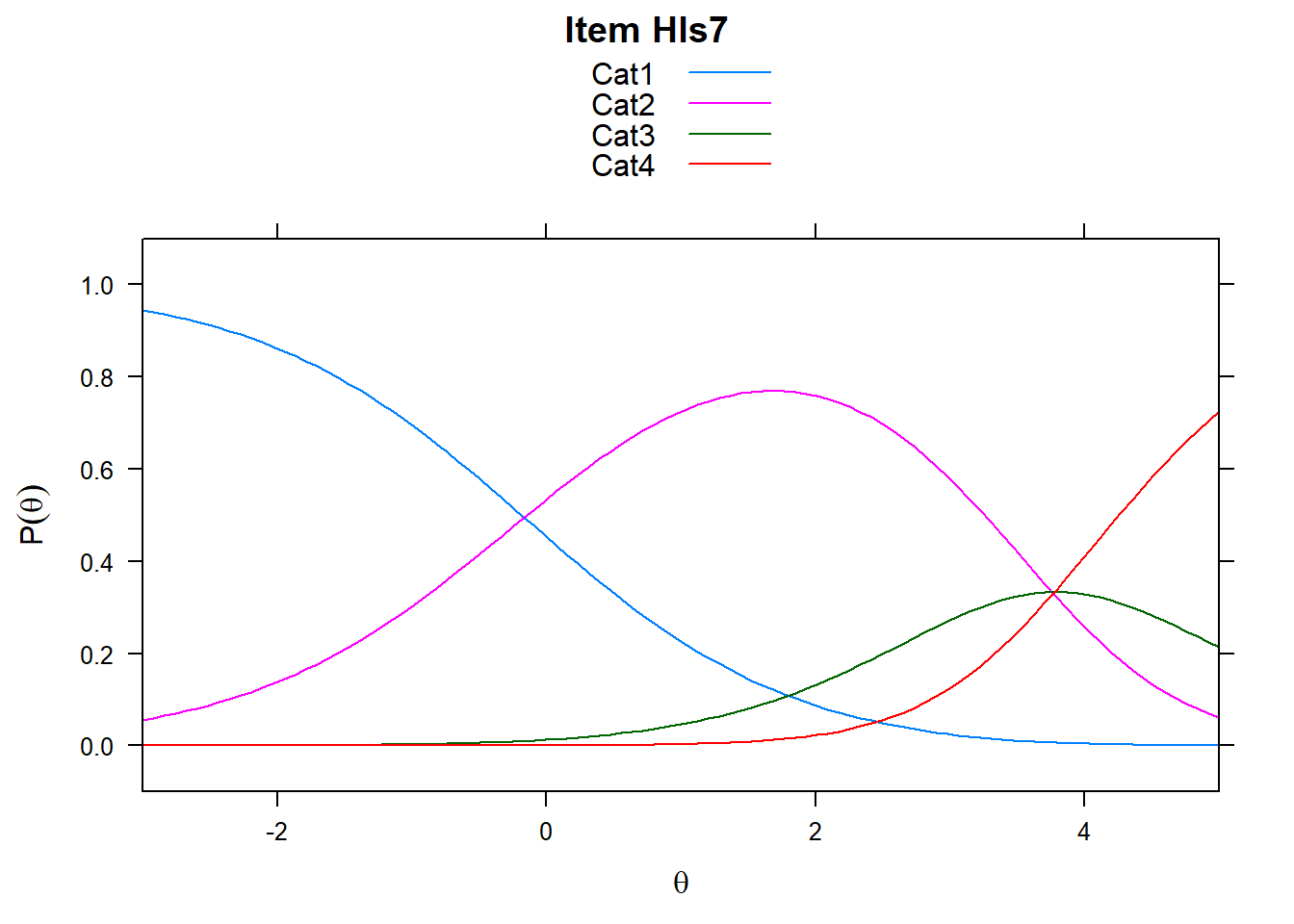
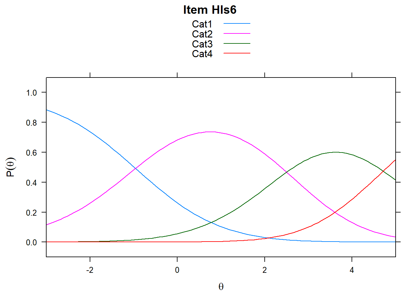
It’s worth remembering what these plots show. The item characteristic curves represent the probability of responding in a particular category given ability. However, xsi, the non-cumulative show the “transition” points - these are the difficulties, or steps. So Cat1 is the first response category in the plot. However, when we look at mod_pcm$xsi or the equivalent, these are the steps.
# just look at a few items - items 5-8
plot(mod_pcm, type = "items", export = F, high = 5, items = c(5:8))
## Iteration in WLE/MLE estimation 1 | Maximal change 2.6967
## Iteration in WLE/MLE estimation 2 | Maximal change 2.1777
## Iteration in WLE/MLE estimation 3 | Maximal change 0.368
## Iteration in WLE/MLE estimation 4 | Maximal change 0.0135
## Iteration in WLE/MLE estimation 5 | Maximal change 3e-04
## Iteration in WLE/MLE estimation 6 | Maximal change 0
## ----
## WLE Reliability= 0.9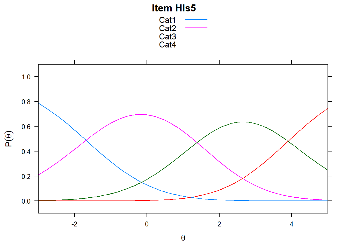
# extract item steps/adjacent category difficulties
xsi_pcm <- mod_pcm$xsi
head(xsi_pcm)
## xsi se.xsi
## Hls1_Cat1 -1.846047 0.1770841
## Hls1_Cat2 2.298335 0.1736858
## Hls1_Cat3 3.830386 0.4635448
## Hls2_Cat1 -1.501716 0.1640914
## Hls2_Cat2 2.764561 0.2004621
## Hls2_Cat3 4.958325 0.7804292# delta-tau
delta_tau_pcm <- mod_pcm$item_irt
head(delta_tau_pcm)## item alpha beta tau.Cat1 tau.Cat2 tau.Cat3
## 1 Hls1 1 1.427471 -3.273603 0.8707754 2.402828
## 2 Hls2 1 2.073633 -3.575436 0.6908362 2.884600
## 3 Hls3 1 2.902846 -3.283771 1.0592760 2.224495
## 4 Hls4 1 2.809263 -2.633376 1.5152151 1.118161
## 5 Hls5 1 1.198341 -2.882556 0.1835035 2.699053
## 6 Hls6 1 1.818401 -2.973840 1.1208579 1.8529825.3.2 Get thresholds
Below, I given an example of how one may acquire thresholds and plot. We have to “pivot” our data into long form to make this feasible. What this means is that, instead of categories going across the top, there’s now one row per each item-threshold pair.
thresh_pcm <- as.data.frame(tam.threshold(mod_pcm))

# transition to long data
thresh_pcm_long <- thresh_pcm %>%
  mutate(item = rownames(.))%>%
  pivot_longer(cols = c(Cat1, Cat2, Cat3))

head(thresh_pcm_long)
## # A tibble: 6 x 3
## item name value
## <chr> <chr> <dbl>
## 1 Hls1 Cat1 -1.86
## 2 Hls1 Cat2 2.15
## 3 Hls1 Cat3 4.00
## 4 Hls2 Cat1 -1.52
## 5 Hls2 Cat2 2.68
## 6 Hls2 Cat3 5.05ggplot(data = thresh_pcm_long, aes(x=item, y=value, colour = name)) + geom_point() +
theme(axis.text.x = element_text(angle = 90))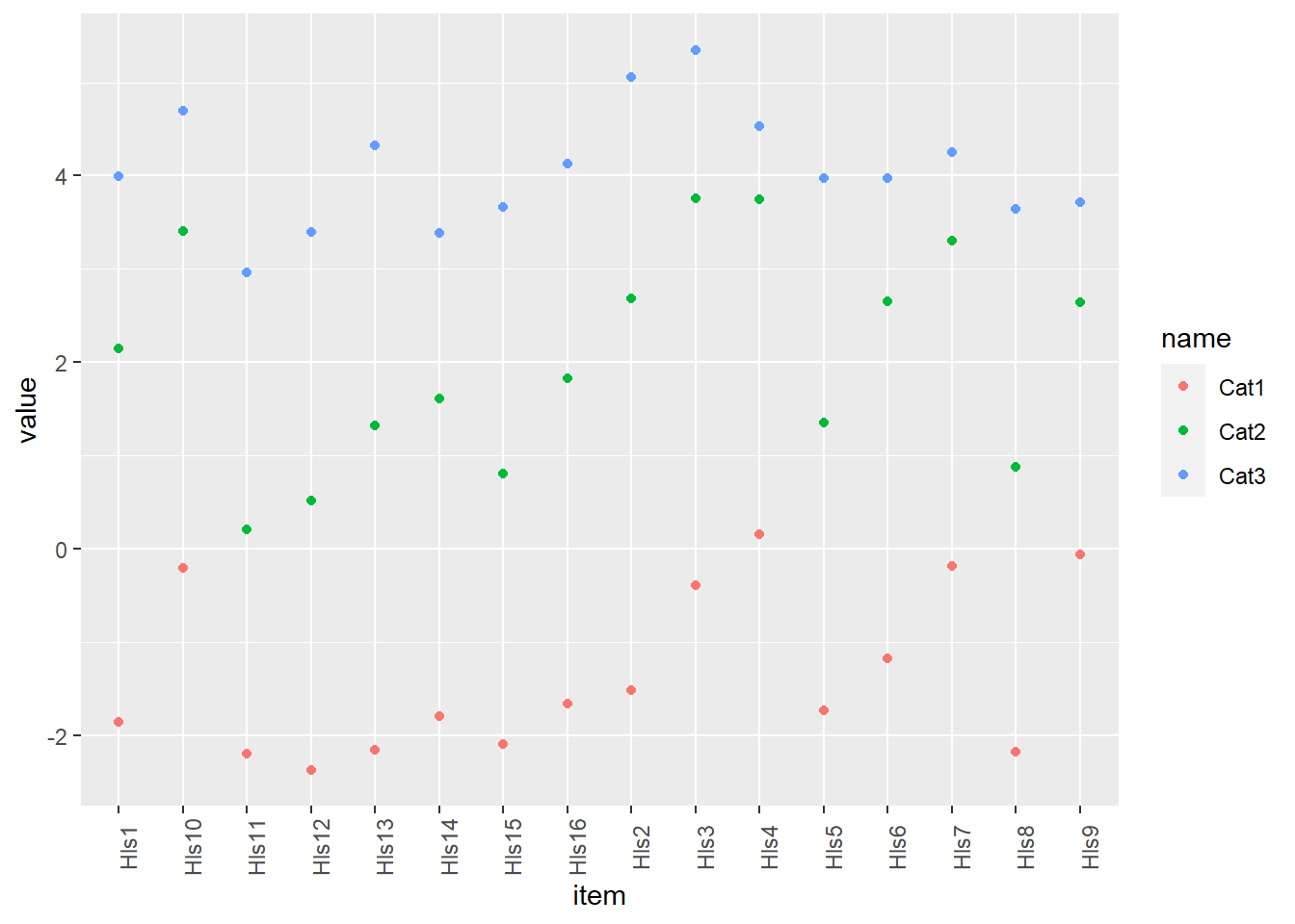
5.3.3 Plotting delta_tau
If you’re interested in plotting a nice item map. This is complicated method for plotting.
delta_tau_p <- delta_tau_pcm %>%
  mutate(d1 = beta + tau.Cat1,
         d2 = beta + tau.Cat2,
         d3 = beta + tau.Cat3) %>% #create the deltas to get overall difficulty
  select(item, beta, d1, d2, d3) %>% # keep just what's important
  mutate(beta_diff = beta) %>% # for ordering later - just create a column with overall delta parameter/mean
  pivot_longer(cols = c(beta, d1, d2, d3), names_to = "Parameter" ) %>% # turn into a long dataframe
  mutate(type_delta = as.factor(if_else(Parameter == "beta", "beta", "delta"))) %>% # for plotting - will color based type_delta
  arrange(beta_diff)

delta_tau_p
## # A tibble: 64 x 5
## item beta_diff Parameter value type_delta
## <fct> <dbl> <chr> <dbl> <fct>
## 1 Hls11 0.325 beta 0.325 beta
## 2 Hls11 0.325 d1 -2.11 delta
## 3 Hls11 0.325 d2 0.173 delta
## 4 Hls11 0.325 d3 2.91 delta
## 5 Hls12 0.512 beta 0.512 beta
## 6 Hls12 0.512 d1 -2.32 delta
## 7 Hls12 0.512 d2 0.513 delta
## 8 Hls12 0.512 d3 3.34 delta
## 9 Hls8 0.781 beta 0.781 beta
## 10 Hls8 0.781 d1 -2.14 delta
## # ... with 54 more rows# this is pretty complicated, sorry...
#but try removing and replacing different lines of code
# to see how it works
pcmp <- ggplot(delta_tau_p, aes(x = reorder(item, beta_diff), # ordering difficulties by beta
y = value, #what's on the y-axis
group = item, # the line segments need to "know" where to connect
fill=type_delta, # what to fill on
shape = type_delta, # only some shapes are fillable
)) +
geom_point(size = 2)+ # making points a little big
theme_bw() +
scale_fill_manual(values = c("black", "white")) + #have to do this manually - so, two fill colors
scale_shape_manual(values = c(21, 21)) + # http://www.cookbook-r.com/Graphs/Shapes_and_line_types/
geom_line(aes(x=item, y=value)) + # add the lines
coord_flip() + #flip so the x-axis is on the y axist
ggtitle("Plot item difficulties in delta_tau for the PCM") +
xlab("Item") +
ylab("Difficulties in logits")
pcmp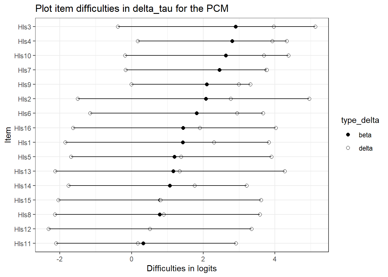
5.4 Running a Rating Scale Model
Now, it doesn’t take a lot to change the model from the partial credit model to the RSM
# Run the rating scale model


mod_rsm <- tam.mml(hls2, irtmodel = "RSM")
5.5 Rating Scale Deltas/thresholds
What are the difficulties in the first form of the partial credit model we learned? Nearly identical.
Note, that for xsi for the rating scale model, you only get one overall item difficulty. This is because the rating scale/taus are the same.
xsi_rsm <- mod_rsm$xsi


#PCM steps/adjacent categories
xsi_pcm[1:10, ]
## xsi se.xsi
## Hls1_Cat1 -1.8460467 0.1770841
## Hls1_Cat2 2.2983348 0.1736858
## Hls1_Cat3 3.8303859 0.4635448
## Hls2_Cat1 -1.5017158 0.1640914
## Hls2_Cat2 2.7645609 0.2004621
## Hls2_Cat3 4.9583249 0.7804292
## Hls3_Cat1 -0.3808346 0.1378983
## Hls3_Cat2 3.9622135 0.3205437
## Hls3_Cat3 5.1274286 1.1165768
## Hls4_Cat1 0.1759761 0.1331498#note the differences - this is the RSM
xsi_rsm## xsi se.xsi
## Hls1 1.5377201 0.10610444
## Hls2 1.9185631 0.10871310
## Hls3 2.8627530 0.11419314
## Hls4 3.3041545 0.11730380
## Hls5 1.1435768 0.10316194
## Hls6 2.0856246 0.10975401
## Hls7 2.9413247 0.11467907
## Hls8 0.6707580 0.09968413
## Hls9 2.8237128 0.11395898
## Hls10 2.9413247 0.11467907
## Hls11 0.1334497 0.09642062
## Hls12 0.3593760 0.09766484
## Hls13 0.9961908 0.10204943
## Hls14 1.2400379 0.10389230
## Hls15 0.6509113 0.09954679
## Hls16 1.4593359 0.10553224
## Cat1 -3.0431277 0.03832376
## Cat2 0.4158395 0.04178431#delta_tau for RSM
mod_rsm$item_irt[1:5, ]## item alpha beta tau.Cat1 tau.Cat2 tau.Cat3
## 1 Hls1 1 1.537630 -3.043111 0.4158464 2.627264
## 2 Hls2 1 1.918472 -3.043111 0.4158464 2.627264
## 3 Hls3 1 2.862659 -3.043111 0.4158464 2.627264
## 4 Hls4 1 3.304060 -3.043111 0.4158464 2.627264
## 5 Hls5 1 1.143488 -3.043111 0.4158464 2.6272645.5.1 Plot the RSM
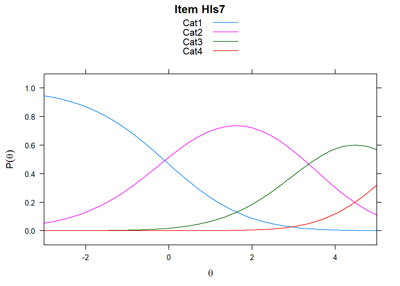
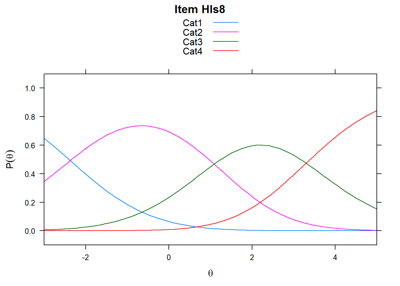
Note the plots below - the item characteristic curves are the same for each category. Note items 7 and 8.
plot(mod_rsm, type = "items", high = 5, items = c(5:8), export = F)## Iteration in WLE/MLE estimation 1 | Maximal change 2.9557
## Iteration in WLE/MLE estimation 2 | Maximal change 2.2955
## Iteration in WLE/MLE estimation 3 | Maximal change 0.3239
## Iteration in WLE/MLE estimation 4 | Maximal change 0.0143
## Iteration in WLE/MLE estimation 5 | Maximal change 4e-04
## Iteration in WLE/MLE estimation 6 | Maximal change 0
## ----
## WLE Reliability= 0.904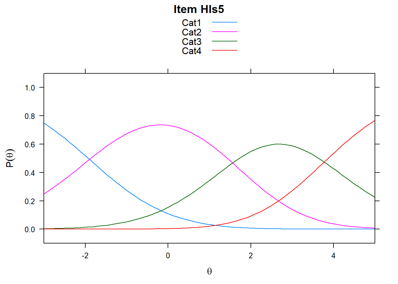
5.5.2 Rating Scale in Delta_Tau vs PCM
What about delta_tau parameterizations comparisons? This is where we might see some differences . . .
These may be the same, but may not. But since the threshold are constrained equality, they might be a different.Here, they’re quite different.
delta_tau_rsm <- mod_rsm$item_irt5.5.3 Comparing the plots of the PCM and RSM
First, need to get the RSM data into the proper form.
delta_tau_r <- delta_tau_rsm %>%
  mutate(d1 = beta + tau.Cat1,
         d2 = beta + tau.Cat2,
         d3 = beta + tau.Cat3) %>%
  select(item, beta, d1, d2, d3) %>%
  mutate(beta_diff = beta) %>%
  pivot_longer(cols = c(beta, d1, d2, d3), names_to = "Parameter" ) %>%
  mutate(type_delta = as.factor(if_else(Parameter == "beta", "beta", "delta"))) %>%
  arrange(beta_diff)

delta_tau_r[1:10, ]
## # A tibble: 10 x 5
## item beta_diff Parameter value type_delta
## <fct> <dbl> <chr> <dbl> <fct>
## 1 Hls11 0.133 beta 0.133 beta
## 2 Hls11 0.133 d1 -2.91 delta
## 3 Hls11 0.133 d2 0.549 delta
## 4 Hls11 0.133 d3 2.76 delta
## 5 Hls12 0.359 beta 0.359 beta
## 6 Hls12 0.359 d1 -2.68 delta
## 7 Hls12 0.359 d2 0.775 delta
## 8 Hls12 0.359 d3 2.99 delta
## 9 Hls15 0.651 beta 0.651 beta
## 10 Hls15 0.651 d1 -2.39 delta5.5.4 Plot the RSM and the PCM!
rsmp <- ggplot(delta_tau_r, aes(x = reorder(item, beta_diff),
                        y = value, #what's on the y-axis
                        group = item, # the line segments need to "know" where to connect
                        fill=type_delta,
                        shape = type_delta, # only some shapes are fillable
                        )) +
  geom_point(size = 2)+ # making points a little big
  theme_bw() +
  scale_fill_manual(values = c("black", "white")) +
  scale_shape_manual(values = c(21, 21)) +
  geom_line(aes(x=item, y=value)) + # add the lines
  coord_flip() + #flip so the x-axis is on the y axist
  ggtitle("Plot item difficulties in delta_tau for the RSM") +
  xlab("Item") +
  ylab("Difficulties in logits")

# RSM
rsmp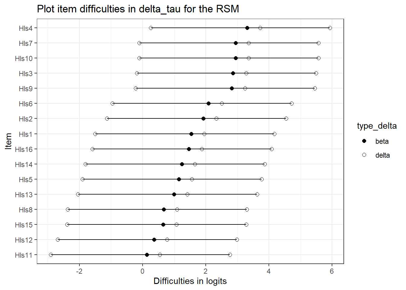
#PCM
pcmp
5.6 Abilities and thresholds
For comparison sakes, let’s compare ability estimates from the two models, RSM and PCM
#PCM
abil_PCM <- tam.wle(mod_pcm)
abil_RSM <- tam.wle(mod_rsm)

thresh_pcm <- tam.threshold(mod_pcm)
thresh_rsm <- tam.threshold(mod_rsm)
5.7 Compare Wrightmaps
WrightMap::wrightMap(thetas = abil_PCM$theta, thresholds = thresh_pcm,
                     main.title = "WrightMap for PCM", return.thresholds = F)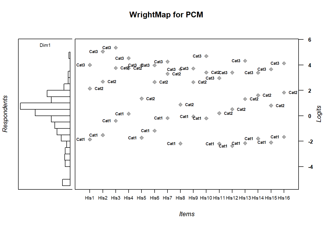
WrightMap::wrightMap(thetas = abil_RSM$theta, thresholds = thresh_rsm,
                     main.title = "WrightMap for RSM", return.thresholds = F)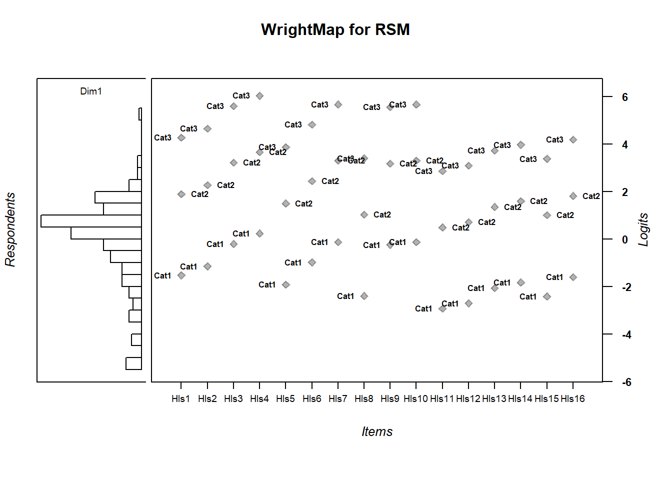
5.8 Compare Item fit
Note, the rating scale model in TAM has a specific parameterization so you have these general category fit stats as well, but they’re not that informative here.
Note, because there is some simulation involved here, you may get different values. Most notably, because of the extremely sparse responses in certain categories, you’ll get strange values.
Note, for the rating scale fit, you really only get overall item fit from TAM.
# PCM

fit_PCM <- tam.fit(mod_pcm)

fit_RSM <- tam.fit(mod_rsm)

#PCM
head(fit_PCM$itemfit)

#RSM
head(fit_RSM$itemfit)
5.9 Model Comparison
TAM stores likelihood information in its model fitting procedure. You can access it individually, or, from the CDM package, which loads with TAM, it’ll compare models for you. Just comparing the log likelihoods from the PCM and RSM (you can do this here because the models are nested).
We can also use anova which will give us fit stats.
TAM can compare two of the models it has produced using a likelihood ratio test with the anova function or with IRT.compareModels. IRT.compareModels, along with anova will give you chi-square difference tests between the likelihoods of the two models.
AIC and BIC allow you to compare models while penalizing for model complexity (BIC penalizes more). In general, the model with a smaller AIC/BIC is the one that the data fit better.
In our case, we see that the \(G^2\) (Deviance) is lower for the PCM and this difference is statistically signigicance. However, it’s worth noting that the BIC is is actually lower (and hence implies a better fitting model) for the RSM.
log_lik_RSM <- logLik(mod_rsm)

log_lik_PCM <- logLik(mod_pcm)

# Model comparisons
anova(mod_rsm, mod_pcm)
## Model loglike Deviance Npars AIC BIC
## 1 mod_rsm -4237.477 8474.955 19 8512.955 8584.374
## 2 mod_pcm -4185.626 8371.252 49 8469.252 8653.438
## Chisq df p
## 1 103.7025 30 0
## 2 NA NA NA#
mod_comp <- IRT.compareModels(mod_pcm, mod_rsm)
mod_comp$IC## Model loglike Deviance Npars Nobs AIC BIC
## 1 mod_pcm -4185.626 8371.252 49 317 8469.252 8653.438
## 2 mod_rsm -4237.477 8474.955 19 317 8512.955 8584.374
## AIC3 AICc CAIC
## 1 8518.252 8487.604 8702.438
## 2 8531.955 8515.514 8603.374# Note based on deviance
mod_comp$LRtest## Model1 Model2 Chi2 df p
## 1 mod_rsm mod_pcm 103.7025 30 4.78886e-105.10 Using the eRm Package
Using the Extended Rasch Modeling Package or eRm is nice, but it uses some different parameterizations than TAM and the fact it uses conditional maximum likelihood estimation instead of maximum likelihood. The main goal is to use its plotting functionality.
5.11 eRm: The PCM and RSM
#Run the PCM in eRm

erm_pcm <- PCM(X = hls2, )

erm_RSM <- RSM(X = hls2)
5.11.1 Getting model results
# Get PCM item difficulties/model results
summary(erm_pcm)
##
## Results of PCM estimation:
##
## Call: PCM(X = hls2)
##
## Conditional log-likelihood: -3109.029
## Number of iterations: 227
## Number of parameters: 47
##
## Item (Category) Difficulty Parameters (eta): with 0.95 CI:
## Estimate Std. Error lower CI upper CI
## Hls1.c2 -0.981 0.246 -1.463 -0.498
## Hls1.c3 1.969 0.497 0.994 2.943
## Hls2.c1 -2.170 0.172 -2.507 -1.834
## Hls2.c2 -0.167 0.252 -0.661 0.328
## Hls2.c3 3.943 0.795 2.386 5.501
## Hls3.c1 -1.027 0.140 -1.302 -0.752
## Hls3.c2 2.130 0.340 1.464 2.796
## Hls3.c3 6.457 1.118 4.266 8.648
## Hls4.c1 -0.481 0.135 -0.746 -0.217
## Hls4.c2 3.013 0.405 2.219 3.807
## Hls4.c3 6.159 0.899 4.398 7.920
## Hls5.c1 -2.363 0.190 -2.736 -1.990
## Hls5.c2 -1.681 0.226 -2.125 -1.237
## Hls5.c3 1.354 0.433 0.506 2.203
## Hls6.c1 -1.806 0.160 -2.119 -1.492
## Hls6.c2 0.364 0.258 -0.142 0.870
## Hls6.c3 3.148 0.545 2.079 4.217
## Hls7.c1 -0.812 0.138 -1.083 -0.541
## Hls7.c2 2.125 0.324 1.490 2.760
## Hls7.c3 5.053 0.722 3.637 6.468
## Hls8.c1 -2.877 0.218 -3.305 -2.450
## Hls8.c2 -2.650 0.244 -3.129 -2.171
## Hls8.c3 0.084 0.385 -0.670 0.838
## Hls9.c1 -0.650 0.139 -0.923 -0.376
## Hls9.c2 1.539 0.263 1.024 2.053
## Hls9.c3 3.952 0.505 2.962 4.942
## Hls10.c1 -0.830 0.139 -1.101 -0.558
## Hls10.c2 2.052 0.315 1.434 2.670
## Hls10.c3 5.615 0.850 3.949 7.280
## Hls11.c1 -2.867 0.233 -3.324 -2.410
## Hls11.c2 -3.322 0.253 -3.818 -2.826
## Hls11.c3 -1.230 0.327 -1.871 -0.588
## Hls12.c1 -3.101 0.235 -3.562 -2.640
## Hls12.c2 -3.236 0.257 -3.740 -2.732
## Hls12.c3 -0.726 0.362 -1.436 -0.017
## Hls13.c1 -2.861 0.211 -3.273 -2.448
## Hls13.c2 -2.217 0.242 -2.692 -1.742
## Hls13.c3 1.202 0.489 0.243 2.162
## Hls14.c1 -2.448 0.189 -2.819 -2.077
## Hls14.c2 -1.396 0.234 -1.855 -0.936
## Hls14.c3 0.937 0.378 0.197 1.678
## Hls15.c1 -2.772 0.215 -3.193 -2.350
## Hls15.c2 -2.627 0.241 -3.099 -2.156
## Hls15.c3 0.137 0.383 -0.613 0.886
## Hls16.c1 -2.303 0.182 -2.660 -1.946
## Hls16.c2 -1.121 0.231 -1.574 -0.669
## Hls16.c3 2.031 0.489 1.074 2.989
##
## Item Easiness Parameters (beta) with 0.95 CI:
## Estimate Std. Error lower CI upper CI
## beta Hls1.c1 2.542 0.188 2.173 2.910
## beta Hls1.c2 0.981 0.246 0.498 1.463
## beta Hls1.c3 -1.969 0.497 -2.943 -0.994
## beta Hls2.c1 2.170 0.172 1.834 2.507
## beta Hls2.c2 0.167 0.252 -0.328 0.661
## beta Hls2.c3 -3.943 0.795 -5.501 -2.386
## beta Hls3.c1 1.027 0.140 0.752 1.302
## beta Hls3.c2 -2.130 0.340 -2.796 -1.464
## beta Hls3.c3 -6.457 1.118 -8.648 -4.266
## beta Hls4.c1 0.481 0.135 0.217 0.746
## beta Hls4.c2 -3.013 0.405 -3.807 -2.219
## beta Hls4.c3 -6.159 0.899 -7.920 -4.398
## beta Hls5.c1 2.363 0.190 1.990 2.736
## beta Hls5.c2 1.681 0.226 1.237 2.125
## beta Hls5.c3 -1.354 0.433 -2.203 -0.506
## beta Hls6.c1 1.806 0.160 1.492 2.119
## beta Hls6.c2 -0.364 0.258 -0.870 0.142
## beta Hls6.c3 -3.148 0.545 -4.217 -2.079
## beta Hls7.c1 0.812 0.138 0.541 1.083
## beta Hls7.c2 -2.125 0.324 -2.760 -1.490
## beta Hls7.c3 -5.053 0.722 -6.468 -3.637
## beta Hls8.c1 2.877 0.218 2.450 3.305
## beta Hls8.c2 2.650 0.244 2.171 3.129
## beta Hls8.c3 -0.084 0.385 -0.838 0.670
## beta Hls9.c1 0.650 0.139 0.376 0.923
## beta Hls9.c2 -1.539 0.263 -2.053 -1.024
## beta Hls9.c3 -3.952 0.505 -4.942 -2.962
## beta Hls10.c1 0.830 0.139 0.558 1.101
## beta Hls10.c2 -2.052 0.315 -2.670 -1.434
## beta Hls10.c3 -5.615 0.850 -7.280 -3.949
## beta Hls11.c1 2.867 0.233 2.410 3.324
## beta Hls11.c2 3.322 0.253 2.826 3.818
## beta Hls11.c3 1.230 0.327 0.588 1.871
## beta Hls12.c1 3.101 0.235 2.640 3.562
## beta Hls12.c2 3.236 0.257 2.732 3.740
## beta Hls12.c3 0.726 0.362 0.017 1.436
## beta Hls13.c1 2.861 0.211 2.448 3.273
## beta Hls13.c2 2.217 0.242 1.742 2.692
## beta Hls13.c3 -1.202 0.489 -2.162 -0.243
## beta Hls14.c1 2.448 0.189 2.077 2.819
## beta Hls14.c2 1.396 0.234 0.936 1.855
## beta Hls14.c3 -0.937 0.378 -1.678 -0.197
## beta Hls15.c1 2.772 0.215 2.350 3.193
## beta Hls15.c2 2.627 0.241 2.156 3.099
## beta Hls15.c3 -0.137 0.383 -0.886 0.613
## beta Hls16.c1 2.303 0.182 1.946 2.660
## beta Hls16.c2 1.121 0.231 0.669 1.574
## beta Hls16.c3 -2.031 0.489 -2.989 -1.074# Get Rating Scale data
summary(erm_RSM)##
## Results of RSM estimation:
##
## Call: RSM(X = hls2)
##
## Conditional log-likelihood: -3152.48
## Number of iterations: 14
## Number of parameters: 17
##
## Item (Category) Difficulty Parameters (eta): with 0.95 CI:
## Estimate Std. Error lower CI upper CI
## Hls2 0.226 0.106 0.018 0.434
## Hls3 1.176 0.113 0.954 1.398
## Hls4 1.612 0.117 1.382 1.842
## Hls5 -0.554 0.101 -0.752 -0.356
## Hls6 0.395 0.107 0.185 0.605
## Hls7 1.254 0.114 1.031 1.477
## Hls8 -1.023 0.099 -1.217 -0.829
## Hls9 1.137 0.113 0.916 1.358
## Hls10 1.254 0.114 1.031 1.477
## Hls11 -1.550 0.099 -1.745 -1.356
## Hls12 -1.329 0.099 -1.523 -1.136
## Hls13 -0.701 0.100 -0.897 -0.504
## Hls14 -0.458 0.101 -0.656 -0.259
## Hls15 -1.043 0.099 -1.237 -0.849
## Hls16 -0.238 0.103 -0.439 -0.036
## Cat 2 3.424 0.086 3.254 3.593
## Cat 3 8.945 0.211 8.531 9.359
##
## Item Easiness Parameters (beta) with 0.95 CI:
## Estimate Std. Error lower CI upper CI
## beta Hls1.c1 0.159 0.103 -0.044 0.361
## beta Hls1.c2 -3.106 0.220 -3.537 -2.676
## beta Hls1.c3 -8.469 0.371 -9.195 -7.743
## beta Hls2.c1 -0.226 0.106 -0.434 -0.018
## beta Hls2.c2 -3.876 0.231 -4.329 -3.422
## beta Hls2.c3 -9.623 0.392 -10.390 -8.856
## beta Hls3.c1 -1.176 0.113 -1.398 -0.954
## beta Hls3.c2 -5.775 0.259 -6.283 -5.267
## beta Hls3.c3 -12.472 0.438 -13.331 -11.614
## beta Hls4.c1 -1.612 0.117 -1.842 -1.382
## beta Hls4.c2 -6.648 0.272 -7.180 -6.115
## beta Hls4.c3 -13.781 0.457 -14.677 -12.885
## beta Hls5.c1 0.554 0.101 0.356 0.752
## beta Hls5.c2 -2.316 0.209 -2.725 -1.906
## beta Hls5.c3 -7.283 0.349 -7.966 -6.600
## beta Hls6.c1 -0.395 0.107 -0.605 -0.185
## beta Hls6.c2 -4.214 0.236 -4.677 -3.750
## beta Hls6.c3 -10.130 0.400 -10.915 -9.345
## beta Hls7.c1 -1.254 0.114 -1.477 -1.031
## beta Hls7.c2 -5.931 0.261 -6.444 -5.419
## beta Hls7.c3 -12.707 0.441 -13.572 -11.842
## beta Hls8.c1 1.023 0.099 0.829 1.217
## beta Hls8.c2 -1.377 0.199 -1.768 -0.987
## beta Hls8.c3 -5.875 0.324 -6.510 -5.241
## beta Hls9.c1 -1.137 0.113 -1.358 -0.916
## beta Hls9.c2 -5.698 0.258 -6.203 -5.192
## beta Hls9.c3 -12.356 0.436 -13.211 -11.501
## beta Hls10.c1 -1.254 0.114 -1.477 -1.031
## beta Hls10.c2 -5.931 0.261 -6.444 -5.419
## beta Hls10.c3 -12.707 0.441 -13.572 -11.842
## beta Hls11.c1 1.550 0.099 1.356 1.745
## beta Hls11.c2 -0.323 0.194 -0.704 0.058
## beta Hls11.c3 -4.294 0.300 -4.882 -3.706
## beta Hls12.c1 1.329 0.099 1.136 1.523
## beta Hls12.c2 -0.765 0.195 -1.148 -0.382
## beta Hls12.c3 -4.957 0.309 -5.563 -4.351
## beta Hls13.c1 0.701 0.100 0.504 0.897
## beta Hls13.c2 -2.022 0.206 -2.425 -1.619
## beta Hls13.c3 -6.842 0.341 -7.510 -6.175
## beta Hls14.c1 0.458 0.101 0.259 0.656
## beta Hls14.c2 -2.508 0.211 -2.923 -2.094
## beta Hls14.c3 -7.572 0.354 -8.266 -6.878
## beta Hls15.c1 1.043 0.099 0.849 1.237
## beta Hls15.c2 -1.338 0.199 -1.728 -0.948
## beta Hls15.c3 -5.817 0.323 -6.449 -5.184
## beta Hls16.c1 0.238 0.103 0.036 0.439
## beta Hls16.c2 -2.948 0.218 -3.375 -2.522
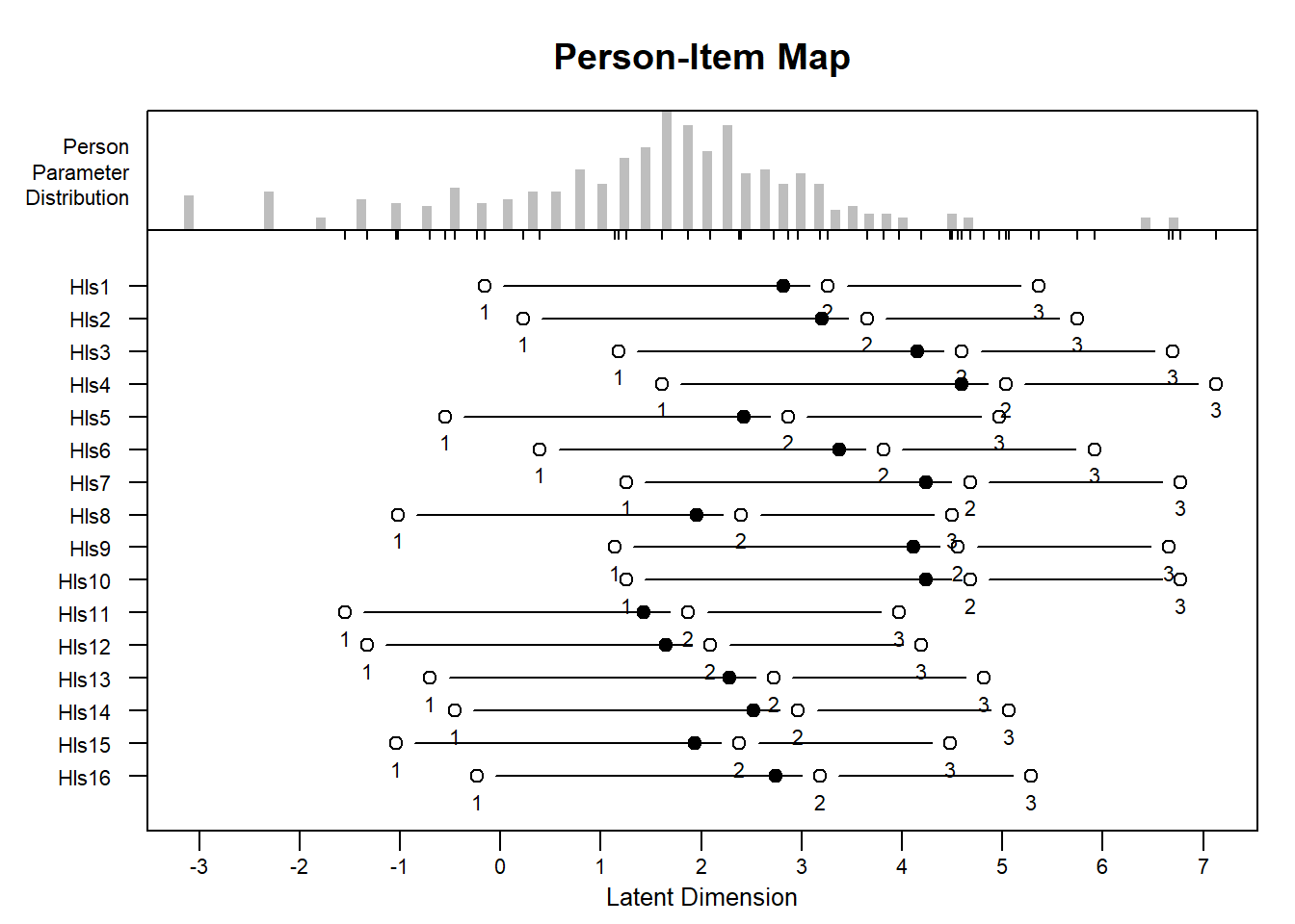
## beta Hls16.c3 -8.232 0.366 -8.950 -7.5145.11.2 Getting item person maps from eRm
Let’s be honest, this is what’s best!
#PCM Item Person Maps
plotPImap(object = erm_pcm)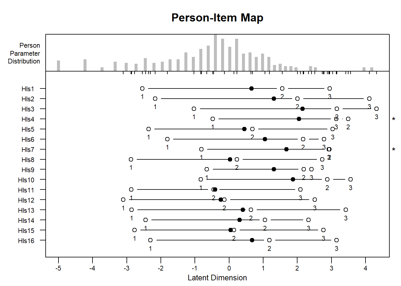
#RSM Item Person Maps
plotPImap(object = erm_RSM)