Chapter 6 Multidimensional Rasch Models
Goals: 1. Learn how to fit and interpret a multidimensional Rasch model 2. Learn how to plot a multidimensional Rasch model 3. Learn how to use basic fit testing to compare the multidimensional Rasch model to the unidimensional model.
6.1 Chapter Workflow
- Fit a unidimensional model
- On the same data, fit a multidimensional model.
- Compare fit.
In this chapter, we’ll learn to fit multidimenstional Rasch models and compare fit of this model to the unidimensional case (a nested model).
The big difference between a multidimensional model and a unidimensional model is that, in the multidimensional model, we are now dealing with multiple latent “traits,” “factors,” “properties,” “constructs” - whatever you want to call them. We usually specify items to “load onto” specific specific properties. We use a matrix, in the TAM called a Q matrix, to describe which factors each item “should”belongs" or “loads.”
There are two types of models: Between-item models - items can only load onto one factor - and within item models where items might load onto multiple factors. We’ll focus on between item models (with correlated factors).
FOr a more in depth introduction, see, Briggs & Wilson (2003)
Warning: Multidimensional models have a strong propensity to fit better than unidimensional models. However, with some strong justification, hopefully in the form of both theorizing and item design, we can combine forms of evidence to justify the model. Fit statistics and the like provide supporting evidence but don’t do any strong confirmation.
Let’s say that we want to measure something like “propensity to be angry” (or something…). You think this data helps you measure this property.
6.2 Data
The data for today comes from commonly used data in learning IRT. The Verbal Aggression Data set. This data is available in the lme4 package. However, I’ve cleaned and subset it as necessary for this lab. The data is dichotomous.
There are 24 items in which respondents answered questions about different scenarios and whether they would curse or shout or scold or merely wanted to (there’s more to it - possible more sources of dimensionality - we won’t deal with that here).
#install.packages(lme4)
library(tidyverse)
library(TAM)
library(WrightMap)
library(lme4)
library(sirt)
6.3 Read in data
If you want to see the data (pre-cleaning), install the lme4 package. Go into the documentation and find the verbAgg dataset that comes with it. We won’t be working with this version.
#pre-cleaned data

#?lme4::VerbAgg

verbal <- read_csv("https://raw.githubusercontent.com/danielbkatz/DBER_Rasch-data/master/data/VerbAgg_multi.csv")
## Parsed with column specification:
## cols(
## .default = col_double()
## )## See spec(...) for full column specifications.# get rid of id column
verb <- verbal[-1]
names(verb)6.4 Comparison: The Unidimensional Rasch Model
We’ll run the same model we’ve been running to set up for comparison.
- Run the Rasch model with the
verbdata. - Get item fit, person abilities.
- Look at person-seperation reliability.
- Make a WrightMap.
We’re going to keep this all stored for comparison later.
# 1. run the model

uni <- tam(verb)

uni_abil <- tam.wle(uni)

uni_fit <- tam.fit(uni)

(eap_rel <- uni$EAP.rel)
6.5 The Multidimensional Rasch Model
Imagine that we’re in the scenario that you think, because some of your items are about wanting to do something and actually doing something (want vs do), that you think there are some people who have divergent scores. That is, there are some people who might have high “ability” on one dimension but not the other. However, you think the dimensions are related and, overall, comprise anger. Alternatively, dimensionality assessment may help you make certain decisions differently if you treat something as multidimensional.
We, however, still want to test the hypothesis that this is a multidimensional measure. However, note, results alone won’t tell us if any dimensionality “found” or not is really just a feature of the instrument and what might be a feature of the property of interest. For instance, negatively worded items may lead us to accept dimensionality whereas it’s a “method effect” and not necessary a feature of the property of interest.
6.6 Setting up the Q Matrix
To do this, we need to set up a Q matrix. We want to have all of the “Wanting” items and all of the doing" items on one dimension.
That is, we need to set up a matrix that has 24 rows and two columns. In column 1, a 1 will represent all the items that are associate with dimension 1 (we’ll make this “want”) and zero otherwise. Column 2, a 1 will be in the place of all items that are associated/load onto dimension 2 (we will call it “want”) and zero otherwise.
6.6.1 Ways to generate the matrix.
- Create a list of 1s and 0 and turn it into a matrix.
- Create a matrix of zeros, use indexing to add correct 1s and zero.
I prefer method 2. But I’ll show you both.
6.6.1.1 Method 1:
names(verb)## [1] "S1WantCurse" "S1WantScold" "S1WantShout" "S2WantCurse"
## [5] "S2WantScold" "S2WantShout" "S3WantCurse" "S3WantScold"
## [9] "S3WantShout" "S4wantCurse" "S4WantScold" "S4WantShout"
## [13] "S1DoCurse" "S1DoScold" "S1DoShout" "S2DoCurse"
## [17] "S2DoScold" "S2DoShout" "S3DoCurse" "S3DoScold"
## [21] "S3DoShout" "S4DoCurse" "S4DoScold" "S4DoShout"Q1 <- matrix(data=c(rep(1, times=12), rep(0, times=12),rep(0, times=12), rep(1, times=12)), ncol=2)
# same as
Q2 <- matrix(c( 1, 1, 1, 1, 1, 1, 1, 1, 1, 1, 1, 1, 0, 0, 0, 0, 0, 0, 0, 0, 0, 0, 0, 0,
0, 0, 0, 0, 0, 0, 0, 0, 0, 0, 0, 0, 1, 1, 1, 1, 1, 1, 1, 1, 1, 1, 1, 1),
ncol=2, nrow = 24)6.6.1.2 Method 2
Method 1 might be best when you have consecutive items like we do (the first 12 go on factor 1, next 12, factor 2). But when things get messier, it’s not so nice. So, it’s easier to generate a matrix and then fill it in.
# create a matrix of just zeros
Q3 <- matrix(0, nrow=24, ncol=2)


#Fill it in
Q3[1:12, 1] <- Q3[13:24, 2] <- 1

# what about if things were not sequential?

Q_rand <- matrix(0, nrow=24, ncol=2)

Q_rand[c(1, 3, 6, 10, 14:17), 1] <- Q_rand[c(2,4,5,7:9, 11:13, 18:24), 2] <- 1
Of course, making matrices isn’t unique to TAM matrices are often useful.
6.7 Run the Multidimensional Rasch Model
multi <- tam(verb, Q=Q3)summary(multi)## ------------------------------------------------------------
## TAM 3.5-19 (2020-05-05 22:45:39)
## R version 3.6.0 (2019-04-26) x86_64, mingw32 | nodename=LAPTOP-K7402PLE | login=katzd
##
## Date of Analysis: 2021-03-05 08:50:29
## Time difference of 1.138995 secs
## Computation time: 1.138995
##
## Multidimensional Item Response Model in TAM
##
## IRT Model: 1PL
## Call:
## tam.mml(resp = resp, Q = ..1)
##
## ------------------------------------------------------------
## Number of iterations = 33
## Numeric integration with 441 integration points
##
## Deviance = 7980.32
## Log likelihood = -3990.16
## Number of persons = 316
## Number of persons used = 316
## Number of items = 24
## Number of estimated parameters = 27
## Item threshold parameters = 24
## Item slope parameters = 0
## Regression parameters = 0
## Variance/covariance parameters = 3
##
## AIC = 8034 | penalty=54 | AIC=-2*LL + 2*p
## AIC3 = 8061 | penalty=81 | AIC3=-2*LL + 3*p
## BIC = 8136 | penalty=155.41 | BIC=-2*LL + log(n)*p
## aBIC = 8050 | penalty=69.43 | aBIC=-2*LL + log((n-2)/24)*p (adjusted BIC)
## CAIC = 8163 | penalty=182.41 | CAIC=-2*LL + [log(n)+1]*p (consistent AIC)
## AICc = 8040 | penalty=59.25 | AICc=-2*LL + 2*p + 2*p*(p+1)/(n-p-1) (bias corrected AIC)
## GHP = 0.52969 | GHP=( -LL + p ) / (#Persons * #Items) (Gilula-Haberman log penalty)
##
## ------------------------------------------------------------
## EAP Reliability
## Dim1 Dim2
## 0.827 0.841
## ------------------------------------------------------------
## Covariances and Variances
## V1 V2
## V1 2.098 1.879
## V2 1.879 2.804
## ------------------------------------------------------------
## Correlations and Standard Deviations (in the diagonal)
## V1 V2
## V1 1.448 0.775
## V2 0.775 1.674
## ------------------------------------------------------------
## Regression Coefficients
## V1 V2
## [1,] 0 0
## ------------------------------------------------------------
## Item Parameters -A*Xsi
## item N M xsi.item AXsi_.Cat1 B.Cat1.Dim1
## 1 S1WantCurse 316 0.712 -1.250 -1.250 1
## 2 S1WantScold 316 0.601 -0.581 -0.581 1
## 3 S1WantShout 316 0.513 -0.086 -0.086 1
## 4 S2WantCurse 316 0.788 -1.786 -1.786 1
## 5 S2WantScold 316 0.627 -0.727 -0.727 1
## 6 S2WantShout 316 0.500 -0.016 -0.016 1
## 7 S3WantCurse 316 0.595 -0.545 -0.545 1
## 8 S3WantScold 316 0.373 0.699 0.699 1
## 9 S3WantShout 316 0.241 1.560 1.560 1
## 10 S4wantCurse 316 0.690 -1.108 -1.108 1
## 11 S4WantScold 316 0.434 0.354 0.354 1
## 12 S4WantShout 316 0.313 1.065 1.065 1
## 13 S1DoCurse 316 0.712 -1.322 -1.322 0
## 14 S1DoScold 316 0.570 -0.402 -0.402 0
## 15 S1DoShout 316 0.342 0.968 0.968 0
## 16 S2DoCurse 316 0.655 -0.935 -0.935 0
## 17 S2DoScold 316 0.487 0.087 0.087 0
## 18 S2DoShout 316 0.247 1.622 1.622 0
## 19 S3DoCurse 316 0.459 0.255 0.255 0
## 20 S3DoScold 316 0.244 1.646 1.646 0
## 21 S3DoShout 316 0.092 3.207 3.207 0
## 22 S4DoCurse 316 0.627 -0.752 -0.752 0
## 23 S4DoScold 316 0.427 0.443 0.443 0
## 24 S4DoShout 316 0.180 2.172 2.172 0
## B.Cat1.Dim2
## 1 0
## 2 0
## 3 0
## 4 0
## 5 0
## 6 0
## 7 0
## 8 0
## 9 0
## 10 0
## 11 0
## 12 0
## 13 1
## 14 1
## 15 1
## 16 1
## 17 1
## 18 1
## 19 1
## 20 1
## 21 1
## 22 1
## 23 1
## 24 1Note, looking at the ouput, we get a bit more than normal: 1. Factor/dimension - Variance-Covariance Matrix (VCV) 2. Factor/dimension correlation matrix 3. Multiple EAP reliabilities for each person (one for each dimension)
6.7.0.1 Person Abilities
multi_abil <- tam.wle(multi)## Iteration in WLE/MLE estimation 1 | Maximal change 1.4551
## Iteration in WLE/MLE estimation 2 | Maximal change 0.6882
## Iteration in WLE/MLE estimation 3 | Maximal change 0.0895
## Iteration in WLE/MLE estimation 4 | Maximal change 0.0149
## Iteration in WLE/MLE estimation 5 | Maximal change 0.003
## Iteration in WLE/MLE estimation 6 | Maximal change 6e-04
## Iteration in WLE/MLE estimation 7 | Maximal change 1e-04
## Iteration in WLE/MLE estimation 8 | Maximal change 0
##
## -------
## WLE Reliability (Dimension1)=0.726
## WLE Reliability (Dimension2)=0.746multi_abil #note, two error variances, two means, two WLE reliability, two variances## Object of class 'tam.wle'
## Call: tam.wle(tamobj = multi)
##
## WLEs for 316 observations and 2 dimensions
##
## WLE Reliability (Dimension 1)=0.726
## Average error variance (Dimension 1)=0.684
## WLE mean (Dimension 1)=-0.011
## WLE variance (Dimension 1)=2.501
##
## WLE Reliability (Dimension 2)=0.746
## Average error variance (Dimension 2)=0.802
## WLE mean (Dimension 2)=0.009
## WLE variance (Dimension 2)=3.158# if you don't want to keep that other WLE info in multi_abil
#df_m_abil <- multi_abil
# class(df_m_abil) <- class(df_m_abil)[2]
ll <- multi$like
## EAP reliabilities
multi$EAP.rel## Dim1 Dim2
## 0.8271830 0.8410392## correlations
variance <- multi$variance
cov2cor(variance)## V1 V2
## V1 1.0000000 0.7747392
## V2 0.7747392 1.00000006.7.0.2 Item fit
multi_fit <- tam.fit(multi)## Item fit calculation based on 100 simulations
## |**********|
## |----------|6.7.0.3 Wright Map
# get thresholds
multi_thresh <- tam.threshold(multi)

#get abilities (you need to subset with the right thetas)

m_theta <- multi_abil[7:8]


wrightMap(thetas = m_theta, thresholds = multi_thresh,
          show.thr.lab = FALSE,
          breaks=15, dim.name=c("want", "do"),
          label.items.srt = 90, axis.persons = "Aggression",
          return.thresholds =F)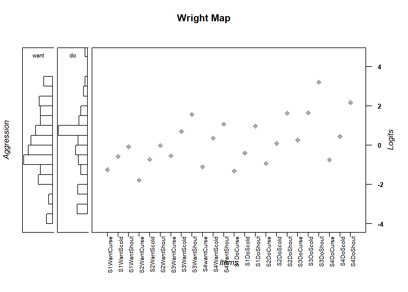
# par(mar = c(bottom, left, top, right))

##par(mar = c(2.1, 4.1, 2.1, 2.1))

# dev.new(width=10, height=10)

wrightMap(thetas = m_theta, thresholds = multi_thresh,
          thr.lab.text = rownames(multi_thresh),
          breaks=15, dim.name=c("want", "do"),
          label.items = "", axis.persons = "Aggression",
          label.items.ticks = FALSE,
          return.thresholds =F)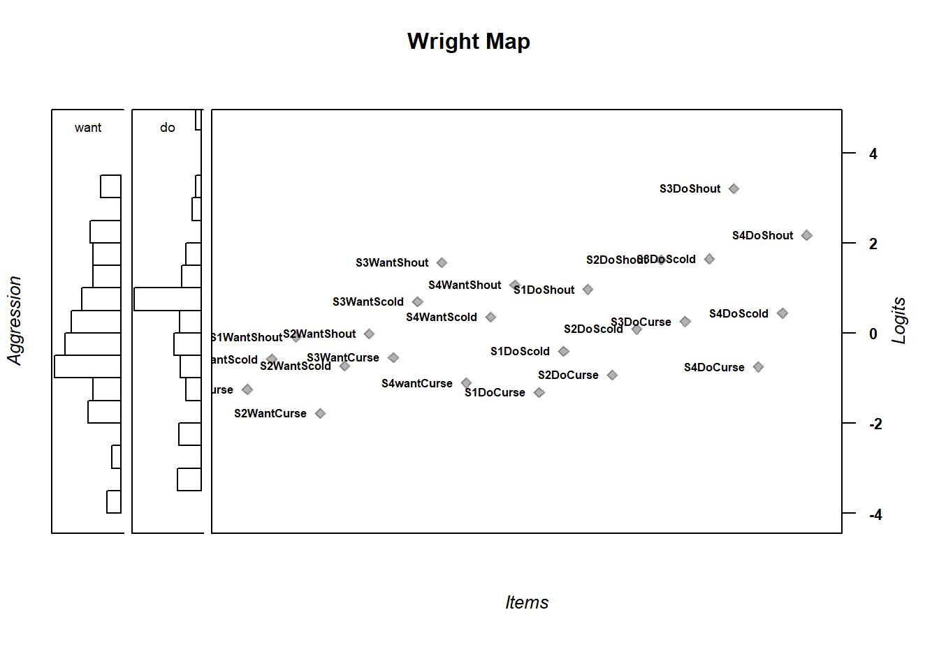
#dev.off()
#graphics.off()

# par("oma") (bottom, left, top, right) in lines

#old.par <- par(mar = c(0, 0, 0, 0))
#par(old.par)

#dev.new(width=10, height=10)

wrightMap(thetas = m_theta, thresholds = multi_thresh,
           item.side = itemClassic, item.prop = .5,
          thr.lab.text = rownames(multi_thresh),
          return.thresholds =F)


wrightMap(thetas = m_theta, thresholds = multi_thresh,
           item.side = itemClassic, item.prop = .5,
          thr.lab.text = rownames(multi_thresh),
          return.thresholds =F)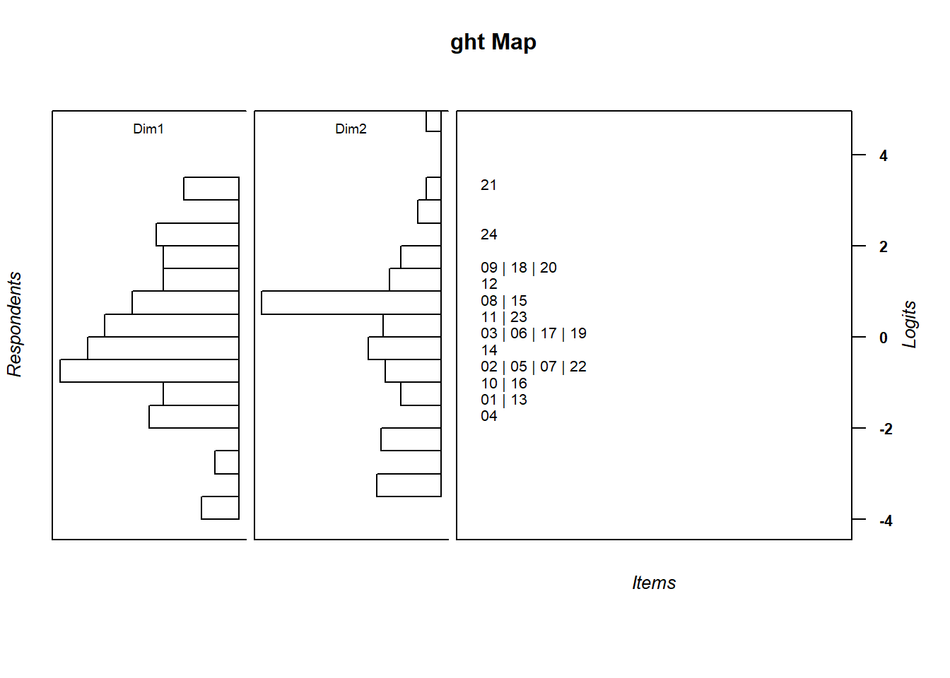
6.7.0.4 Saving
png("Plots/wrightmap.png", width=750)

wrightMap(thetas = m_theta, thresholds = multi_thresh,
           item.side = itemClassic,
          return.thresholds =F, main.title = "Aggression WrightMap",
          )
dev.off()

itemClassic(thr = multi_thresh)
6.8 Comparing model fit
We’ll compare the fit of the two models. Remember we can access these directly.
# get information criteria from the models
uni$ic
## n deviance loglike logprior logpost Nparsxsi NparsB
## 1 316 8073.815 -4036.907 0 -4036.907 24 0
## Nparsbeta Nparscov np Npars ghp_obs AIC AIC3
## 1 0 1 25 25 7584 8123.815 8148.815
## BIC aBIC CAIC AICc GHP
## 1 8217.708 8138.098 8242.708 8128.298 0.5355891multi$ic## n deviance loglike logprior logpost Nparsxsi NparsB
## 1 316 7980.318 -3990.159 0 -3990.159 24 0
## Nparsbeta Nparscov np Npars ghp_obs AIC AIC3
## 1 0 3 27 27 7584 8034.318 8061.318
## BIC aBIC CAIC AICc GHP
## 1 8135.723 8049.745 8162.723 8039.568 0.5296887# compare - which one is "significantly better"
anova(uni, multi)## Model loglike Deviance Npars AIC BIC Chisq
## 1 uni -4036.907 8073.815 25 8123.815 8217.708 93.49644
## 2 multi -3990.159 7980.318 27 8034.318 8135.723 NA
## df p
## 1 2 0
## 2 NA NA# From the CDM package
compares <- IRT.compareModels(uni, multi)
#comparison statistics
compares$IC## Model loglike Deviance Npars Nobs AIC BIC
## 1 uni -4036.907 8073.815 25 316 8123.815 8217.708
## 2 multi -3990.159 7980.318 27 316 8034.318 8135.723
## AIC3 AICc CAIC
## 1 8148.815 8128.298 8242.708
## 2 8061.318 8039.568 8162.723compares$LRtest## Model1 Model2 Chi2 df p
## 1 uni multi 93.49644 2 06.9 manually perform the likelihood ratio/deviance test
# take the deviance differences
devi_diff <- 8073.815-7980.318

df <- 27-25 #npars

# pvalue
1-pchisq(devi_diff, df=df)
## [1] 06.10 Criteria for choosing to use a multidimensional model
Fit is but one way to choose whether to use a multidimensional model or not. There are other, pragmatic considerations. For instance, one may think about how often using a multidimensional model would change the sorts of decisions you would make in a given setting. For instance, perhaps with a unidimensional model, you might see that a student is right in the middle of the ability distribution. However, with multidimensional model, you might see that the student has high ability in one area and low ability in another. This might lead to a different decision in instructional practice.
6.10.1 Activity
Assemble evidence for the model of your choice.
Compare item fit statistcs for both the unidimensional and multidimensional model. Why do you think they’re different?
Would you prefer the two dimensional model or the unidimensional model? Why? (for instance, compare and aggregate fit stats - you may want to export these into a file. EAP Reliability, AIC, BIC, correlations)
Would you want to do do something differently based on what you see or don’t see?
What do you make of the correlations among dimensions?
6.11 Word of Caution for 3 or more dimensions
TAM says:
For more than three dimensions, quasi-Monte Carlo or stochastic integration is recommended because otherwise problems in memory allocation and large computation time will result. Choose in control a suitable value of the number of quasi Monte Carlo or stochastic nodes snodes (say, larger than 1000). See Pan and Thompson (2007) or Gonzales et al. (2006) for more details.
In other words, your computer may start freezing and may never complete estimating a model if you have more than three dimensions (or sometimes fewer). So you have to use ’quasi-Monte Carloorstochastic nodes`. You can change the control options as necessary (I recommend running and changing the maxiter and snodes numbers to see if it changes results drastically)
multi <- tam.mml(resp=verb, Q=Q3, control=list(snodes=2000, maxiter=10))