6 📝 Limit Theorems

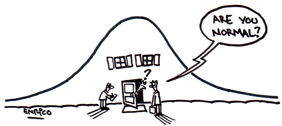
Figure 6.1: ‘AreUnormal’ by Enrico Chavez

6.1 Markov’s and Chebyshev’s Inequalities

We will start by overviewing two inequalities that allow the computation of upper bounds for probability statements and play an important role in stablishing the convergence results we’ll see further in this chapter.

6.1.1 Markov’s inequality

Chebychev’s inequality can be used to construct crude bounds on the probabilities associated with deviations of a random variable from its mean.

6.2 Sequences of Random Variables

We would like to say something about how these random variables behave as \(n\) gets larger and larger (i.e. as \(n\) tends towards infinity, denoted by \(n\rightarrow\infty\) )

The study of such limiting behaviour is commonly called a study of `asymptotics’ — after the word asymptote used in standard calculus.

6.2.1 Example: Bernoulli Trials and their sum

Let \(\tilde Z\) denote a dichotomous random variable with \(\tilde Z\sim \mathcal{B}(p)\). A sequence of Bernoulli trials provides us with a sequence of values \(\tilde Z_{1},\tilde Z_{2},...,\tilde Z_{n},...\) %where each \(\tilde {Z}_{i}\) is such that

\[\begin{eqnarray*} \Pr("Success")=\Pr \left( \tilde{Z}_{i}=1\right) = p & \text{and} & \Pr("Failure")=\Pr \left( \tilde Z_{i}=0\right) = 1-p \end{eqnarray*}\]

Now let \[S_n=\sum_{s=1}^n \tilde Z_s,\] the number of “Successes” in the first \(n\) Bernoulli trials. This yields a new sequence of random variables

\[\begin{eqnarray*} S_{1} &=& \tilde Z_{1} \\ S_{2} &=&\left( \tilde Z_{1}+ \tilde Z_{2}\right)\\ &&\vdots \\ S_{n} &=&\left( \tilde Z_{1}+ \tilde Z_{2}+\cdots + \tilde Z_{n}\right) = \sum_{i=1}^n \tilde Z_i \end{eqnarray*}\]

This new sequence is such that \(S_n\sim B(n,p)\) for each \(n\).

Now consider the sequence:
\[{P}_n=S_n/n,\] for \(n=1,2,\ldots\), corresponds to the proportion of `Successes’in the first \(n\) Bernoulli trials.

It is natural to ask how the behaviour of \({P}_n\) is related to the true probability of a `Success’ (\(p\)).

Specifically, the open question at this point is: \

“Do these results imply that \({P}_n\) collapses onto the true \(p\) as \(n\) increases, and if so, in what way?” \

To gain a clue, let us consider the simulated values of \({P}_n\).

6.2.2 Example: Bernoulli Trials and limit behaviour

So, informally, we can claim that a sequence of random variables \(X_{1},X_{2},...,X_{n},...\) is thought to converge if the probability distribution of \(X_{n}\) gets more and more concentrated around a single point as \(n\) tends to infinity.

6.3 Convergence in Probability (\(\overset{p}{\rightarrow }\))

More formally,

6.3.1 Operational Rules for \(\overset{p}{\rightarrow }\)

Let us itemize some rules. To this end, let \(a\) be any (nonrandom) number so:

• If \(X_{n}\overset{p}{\rightarrow } \alpha\) then

• \(aX_{n}\overset{p}{\rightarrow }a\alpha\) and

• \(a+X_{n}\overset{p}{\rightarrow }a+\alpha\),

• If \(X_{n}\overset{p}{\rightarrow }X\) then

  • \(aX_{n}\overset{p}{\rightarrow }aX\) and
  • \(a+X_{n}\overset{p}{\rightarrow }a+X\)

• If \(X_{n}\overset{p}{\rightarrow }\alpha\) and \(Y_{n}\overset{p}{\rightarrow }\gamma\) then

  • \(X_{n}Y_{n}\overset{p}{\rightarrow }\alpha \gamma\) and
  • \(X_{n}+Y_{n}\overset{p}{\rightarrow }\alpha +\gamma\).

• If \(X_{n}\overset{p}{\rightarrow }X\) and \(Y_{n}\overset{p}{\rightarrow }Y\) then

  • \(X_{n}Y_{n}\overset{p}{\rightarrow }X Y\) and
    
  • \(X_{n}+Y_{n}\overset{p}{\rightarrow }X +Y\)

• Let \(g\left( x\right)\) be any (non-random) continuous function. If \(X_{n}\overset{p}{\rightarrow }\alpha\) then \[g\left( X_{n}\right) \overset{p}{\rightarrow }g\left( \alpha \right),\] and if \(X_{n}\overset{p}{\rightarrow }X\) then

\[g\left( X_{n}\right) \overset{p}{\rightarrow }g\left( X \right).\]

Suppose \(X_{1},X_{2},...,X_{n},...\) is a sequence of random variables with common distribution \(F_X(x)\) and moments \(\mu_r=E [X^r]\). At any given point along the sequence, \(X_{1},X_{2},...,X_{n}\) constitutes a simple random sample of size \(n\). \

For each fixed sample size \(n\), the \(r\)th sample moment is (using an obvious notation) \[\begin{equation*} M_{(r,n)}=\frac{1}{n}\left( X_{1}^r+X_{2}^r+\cdots +X_{n}^r\right)=\frac{1}{n}\sum_{s=1}^nX_s^r\,, \end{equation*}\] and we know that \[E[M_{(r,n)}]=\mu_r\quad\text{and}\quad Var(M_{(r,n)})=\frac{1}{n}(\mu_{2r}-\mu_r^2)\,.\]

Now consider the sequence of sample moments \(M_{(r,1)},M_{(r,2)},...,M_{(r,n)},...\) or, equivalently, \(\{M_{(r,i)}\}_{i=1}^{n}\).

6.3.2 Convergence of Sample Moments as a motivation…

The distribution of \(M_{(r,n)}\) (which is unknown because \(F_X(x)\) has not been specified) is thus concentrated around \(\mu_r\) for all \(n\), with a variance which tends to zero as \(n\) increases. \

So the distribution of \(M_{(r,n)}\) becomes more and more concentrated around \(\mu_r\) as $n $ increases and therefore we might that \[\begin{equation*} M_{(r,n)}\overset{p}{\rightarrow }\mu_r. \end{equation*}\]

In fact, this result follows from what is known as the Weak Law of Large Numbers (WLLN).

6.3.3 The Weak Law of Large Numbers (WLLN)

6.3.4 The WLLN and Chebyshev’s Inequality

• First note that \(E[\overline{Y}_n]=\mu_Y\) and \(Var(\overline{Y}_n)=\sigma_Y^2/n\).
• Now, according to Chebyshev’s inequality \[\begin{eqnarray*} \Pr \left( |\overline{Y}_{n}-\mu_Y| <\varepsilon\right) &\geq &1-\frac{E\left[ \left( \overline{Y}_{n}-\mu_Y \right) ^{2}\right] }{\varepsilon^{2}} \\ &=&1-\frac{\sigma_Y ^{2}/n}{\varepsilon^{2}} \\ &=&1-\frac{\sigma_Y ^{2}}{n\varepsilon^{2}}\geq 1-\delta \end{eqnarray*}\] for all \(n>\sigma_Y^2/(\varepsilon^2\delta)\).
• Thus the WLLN is proven, provided we can verify Chebyshev’s inequality.
• Note that by considering the limit as \(n\rightarrow \infty\) we also have% \[\begin{equation*} \lim_{n\rightarrow \infty }\Pr \left( \left\vert \overline{Y}_{n}-\mu_Y\right\vert <\varepsilon\right) \geq \lim_{n\rightarrow \infty }\left( 1-\frac{\sigma^{2}}{n\varepsilon^{2}}\right) =1\,, \end{equation*}\] again implying that \(\left( \overline{Y}_{n}-\mu_Y \right) \overset{p}{\rightarrow }0\).

• If \(p\lim_{n\rightarrow\infty}(X_n-X)=0\) then \(X_{n}\overset{D}{\rightarrow }X\).

• Let \(a\) be any real number. If \(X_{n}\overset{D}{\rightarrow }X\), then \(aX_{n}\overset{D}{\rightarrow }aX\)

• If \(Y_{n}\overset{p}{\rightarrow }\phi\) and \(X_{n}\overset{D}{% \rightarrow }X\), then

• \(Y_{n}X_{n}\overset{D}{\rightarrow }\phi X,\) and

• \(Y_{n}+X_{n}\overset{D}{\rightarrow }\phi +X\)

• If \(X_{n}\overset{D}{\rightarrow }X\) and \(g\left( x\right)\) is any continuous function, then \(g\left( X_{n}\right) \overset{D}{\rightarrow }% g\left( X\right)\)

The following theorem is often said to be one of the most important results. Its significance lies in the fact that it allows accurate probability calculations to be made without knowledge of the underlying distributions!

%

%