7 📝 Bivariate Discrete Random Variables
Figure 7.1: ‘Correlation’ by Enrico Chavez
7.1 Joint Probability Functions
The joint PMF has two essential properties:
The value of the Joint PMF is always non-negative \[p_{X,Y}\left( x,y\right) \geq 0 \text{ for all possible pairs }\left(x,y\right)\]
The sum over all combinations of \(x\) and \(y\) values is equal to one \[\sum_{x}\sum_{y}\Pr ( \left\{ X=x\cap Y=y\right\}) =1\]
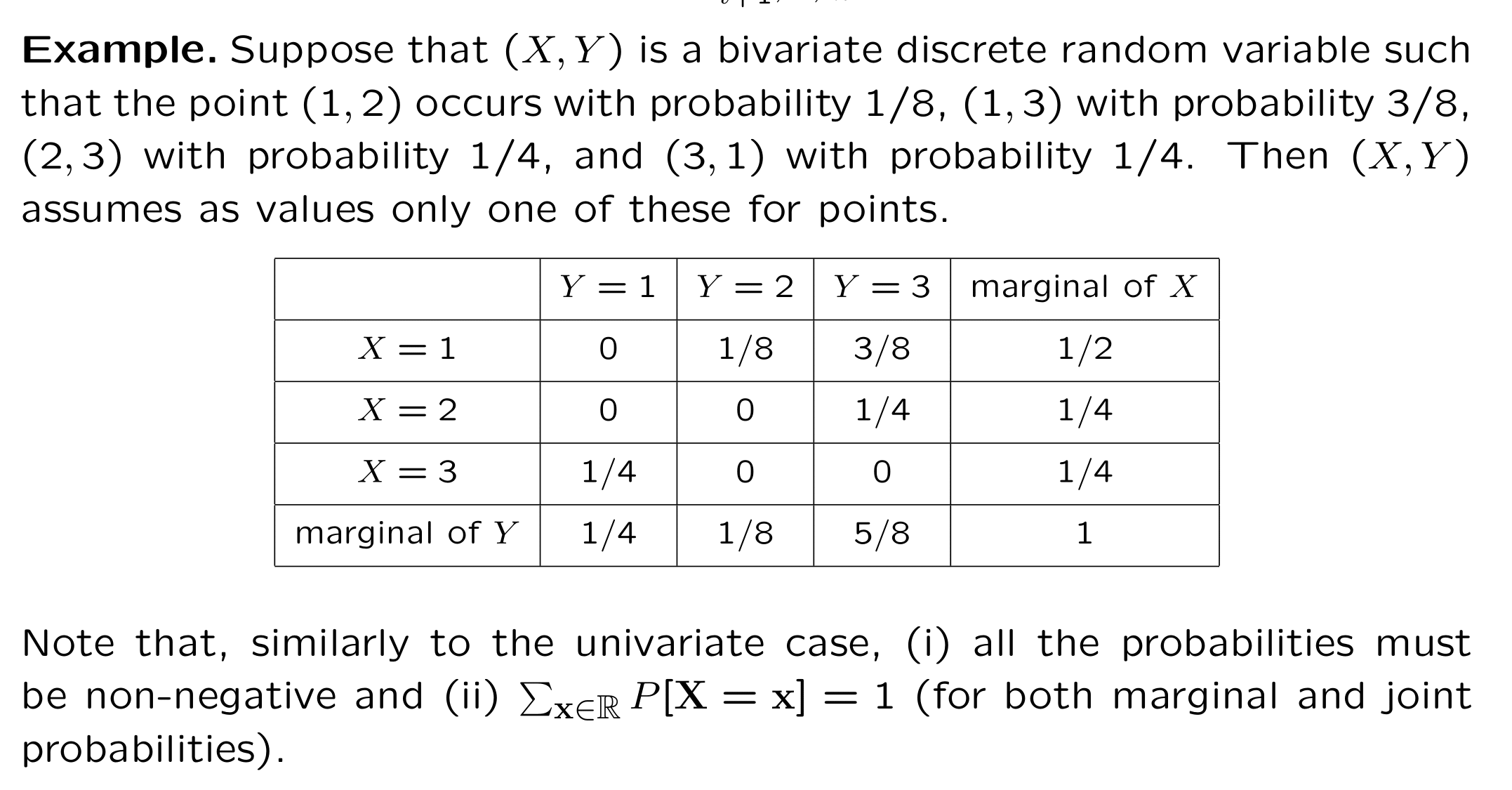
Similarly, the probability (mass) function of the discrete random variable \(Y\) is called its marginal probability (mass) function. It is obtained by summing the joint probabilities relating to pairs \((X,Y)\) over all possible values of \(X\): \[\begin{equation*} p_{Y}(y)=\sum_{x}p_{X,Y}(x,y). \end{equation*}\]
7.2 Conditional Probability
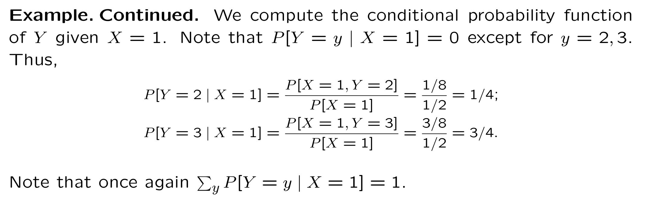
Recall that the conditional probability mass function of the discrete
random variable \(Y\), given that the random variable \(X\) takes the
value \(x\), is given by:
\[\begin{equation*}
p_{Y|X}\left( y|x\right) =\frac{\Pr \left\{ X=x\cap Y=y\right\} }{%
P_{X}\left( X=x\right) }
\end{equation*}\]
Note this is a probability mass function for \(y,\) with \(x\) viewed as fixed. Similarly:
Note this is a probability mass function for \(x,\) with \(y\) viewed as fixed.
7.2.1 Independence
Two discrete random variables \(X\) and \(Y\) are independent if \[\begin{eqnarray*} p_{X,Y}(x,y) &=&p_{X}(x)p_{Y}(y)\qquad \qquad \text{(discrete)} \\ %f_{X,Y}(x,y) &=&f_{X}(x)f_{Y}(y)\qquad \qquad \text{(continuous)} \end{eqnarray*}\] for values of \(x\) and \(y.\)
Note that independence also implies that \[\begin{eqnarray*} p_{X|Y}(x|y) &=&p_{X}(x)\text{ and }p_{Y|X}(y|x)=p_{Y}(y)\qquad \text{ (discrete)} \\ %f_{X|Y}(x|y) &=&f_{X}(x)\text{ and }f_{Y|X}(y|x)=f_{Y}(y)\qquad \text{ %(continuous)} \end{eqnarray*}\] for values of \(x\) and \(y\).
7.3 Expectations
Equivalently, the **conditional expectation }of \(h\left( X,Y\right)\) \(X=x\) is defined as: \[\begin{equation*} E\left[ h\left( X,Y\right) |x\right] =\sum_{y}h\left( x,y\right) p_{Y|X}\left( y|x\right). \end{equation*}\]
7.3.1 Iterated Expectations
This notation emphasises that whenever we write down \(E[\cdot]\) for an expectation we are taking that expectation with respect to the distribution implicit in the formulation of the argument.
The above formula is perhaps more easily understood using the more explicit notation: \[\begin{align*} E_{(X,Y)}[h(X,Y)]&=E_{(Y)}[E_{(X|Y)}[h(X,Y)]]\\ &=E_{(X)}[E_{(Y|X)}[h(X,Y)]] \end{align*}\]
This notation makes it clear what distribution is being used to evaluate the expectation, the joint, the marginal or the conditional.
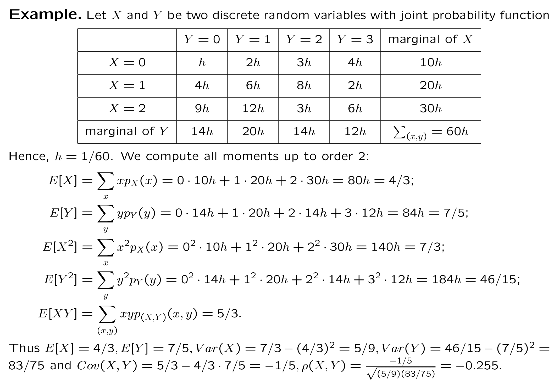
7.4 Covariance and Correlation
Alternative formula1 for \(Cov(X,Y)\) is \[\begin{equation} \boxed{Cov\left( X,Y\right) =E\left[ XY\right] -E\left[ X\right] E\left[ Y\right]\ .} \label{Cov} \end{equation}\]
So, to compute the covariance from a table describing the joint behaviour of \(X\) and \(Y\), you have to:
- compute the joint expectation \(E[XY]\)—you get it making use of the joint probability;
- compute \(E[X]\) and \(E[Y]\)—you get using the marginal probability for \(X\) and \(Y\);
- combine these expected values as in formula ().
See example on page 13 for an illustrative computation.
7.4.1 Some Properties of Covariances
The Cauchy-Schwartz Inequality states \[(E\left[ XY\right])^2\leq E\left[ X^2\right]E\left[ Y^2\right],\] with equality if, and only if, \(\Pr(Y=cX)=1\) for some constant \(c\).
Let \(h(a)=E[(Y-aX)^2]\) where \(a\) is any number. Then \[0\leq h(a)=E[(Y-aX)^2]=E[X^2]a^2-2E[XY]a+E[Y^2]\,.\]
This is a quadratic in \(a\), and
- if \(h(a)>0\) the roots are real and \(4(E[XY])^2-4E[X^2]E[Y^2]<0\),
- if \(h(a)=0\) for some \(a=c\) then \(E[(Y-cX)^2]=0\), which implies that \(\Pr(Y-cX=0)=1\).
Building on this remark, we have \(Cov(X,Y)>0\) if
large values of \(X\) tend to be associated with large values of \(Y\)
small values of \(X\) tend to be associated with small values of \(Y\)
\(Cov(X,Y)<0\) if
large values of \(X\) tend to be associated with values of \(Y\)
small values of \(X\) tend to be associated with values of \(Y\)
When \(Cov(X,Y)=0\), \(X\) and \(Y\) are said to be uncorrelated.
If \(X\) and \(Y\) are two random variables (either discrete or continuous) with \(Cov(X,Y) \neq 0\), then: \[\begin{equation} Var(X + Y) = Var(X) + Var(Y) + 2 Cov(X,Y) \label{FullVar} \end{equation}\]
, where we read that in the case of independent random variables \(X\) and \(Y\) we have \[Var(X + Y) = Var(X) + Var(Y),\] which trivially follows from ()—indeed, for independent random variables, \(Cov(X,Y)\equiv 0\).
- The covariance depends upon the unit of measurement.
7.4.2 A remark
- If we scale \(X\) and \(Y\), the covariance changes: For \(a,b>0\)% \[\begin{equation*} Cov\left( aX,bY\right) =abCov\left( X,Y\right) \end{equation*}\]
Thus, we introduce the correlation between \(X\) and \(Y\) is \[\begin{equation*} corr\left( X,Y\right) =\frac{Cov\left( X,Y\right) }{\sqrt{Var\left( X\right) Var\left( Y\right) }} \end{equation*}\]
which depend upon the unit of measurement.