1 Introduction
Figure 1.1: Taking statistics to schools by Enrico Chavez
1.1 A World of Data
Data is the most important commodity in our connected world of today. Generated at a breakneck pace and related to practically all of the aspects of human life, Data has become a valuable resource for the creation of products and services designed to improve people’s lives. Gathering this data can potentially help companies design better policies and companies design better products.
To illustrate this point, take a look at the following interactive map of the internal migration in Switzerland in 2016. Seizing historical data like this could help decision makers, such as politicians or managers in housing firms, identify migration trends and inform their decisions in what pertains, say housing projects or other infrastructure investments.
Figure 1.2: Inter-cantonal migration in Switzerland in 2016, an interactive map by Ilya Bobadin with data from the Swiss Federal Statistical Office. https://flowmap.blue/.
In order to make sense of the immense amounts of information generated every millisecond, computational tools are needed. Thankfully, in this day and age, computing power allows easy and fast manipulation of that enormous amount of information, and more and more sophisticated algorithms are designed to analyse it, yet it is not only by “brute force” i.e. algorithmic power that appropriate insights are found. To make sense of the data, we also need to consider its features from a mathematical standpoint.
The field of Mathematics that provides a formal framework of the data generation process the field of Probability, and it is the building block for Statistics, the domain of knowledge that deals with the creation of mathematical tools to analyse data.
1.2 What to expect from this Lecture?
In this course, we study Probability as a way to introduce Statistics.
Thus we do not study Probability as a subject of interest in itself. This means that we do not develop deep probability theory using all the formal theoretical arguments, but rather we set up a few principles and methods which will be helpful to study Statistics.
Hence, for the purposes of this lecture, we shall consider:
Statistics: as the discipline that deals with the collection, presentation, analysis and interpretation of data. In future Classes, you will learn classical Statistical methods as well as their modern reincarnation (or “rebranding”): algorithmic tools known as Machine Learning, Deep Learning, etc.
Probability as the mathematical formalisation of randomness and uncertainty the main building block of Statistical methods.
](https://i.redd.it/8r2fd78pgna51.png)
Figure 1.3: Thinking of learning ML this weekend, is there math? (2020). Retrieved from r/DataScienceMemes
1.2.1 One intuitive illustration
Before jumping into the core of the subject, I would like to make a little detour that helps illustrate how prevalent probabilities are in practically every aspect of daily life. Oftentimes, in Movies and TV shows, we hear characters facing uncertain outcomes. When our protagonists are about to make life altering decisions they often ask themselves:
What are my chances of winning?
To which some other character replies with some phrase like:
“I’d say more like one out of a million.”
In your mind, this number becomes an indication of the likelihood of the event happening.
“So, you’re telling me that THERE IS A CHANCE!”
Intuitively, you understand this as the result of the following rationale: were you to repeat the experiment, your “chances of success” result from a ratio between the number of times you succeed, versus the number of attempts.
\[\text{my chances} = \frac{\text{number of times I succeed}}{\text{number of times I fail}}\] In a bit of an abuse of language, this value, constitutes the probability of success.
When it’s small, success is very unlikely, but if it is large (or at least closer to 1), your success seems more likely, as the times you succeed in the experiments are more frequent.
Probability constitutes then the measure of the “likelihood” of an event or random outcome.
“In this world there is nothing certain but death and taxes.”
— Benjamin Franklin
1.2.1.1 Another illustration: Stock price evolution
Let us see how to characterise the uncertainty of the price of a financial asset, such as a Stock, with a simple probabilistic model. To account for the fluctuations in the price, we can make the following simple assumptions:
Let \(S_0\) denote the price of the Stock at time \(t_0\), and consider that:
- with probability \(p\) the stock price increases by a factor \(u>1\), and
- with probability \(1-p\) the price goes down a factor \(d<1\).
We can therefore infer the price at time \(t_1\) by \(S_1 = uS_0\) if the price goes up, and by \(S_1=dS_0\) if the price goes down.
Let us set \(S_0=1\) (US Dollar) and the factors \(u=2\) (i.e. doubling the price) and \(d=1/2\) (i.e. halving the price). What can we say about the price at time \(t_2\)?
To answer this last question we could represent the evolution of the price using a Probability Tree Diagram. In such charts, we organise the different outcomes in branches. At the end of each branch (in the nodes) , we place the outcomes while, hovering over each branch (on the edges) we place the probability associated with the outcome.
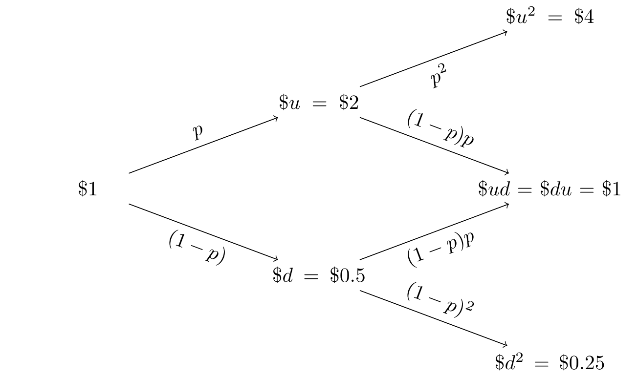
Figure 1.4: Stock Price Evolution as a Probability Tree Diagram
- To compute the probability of successive outcomes, we multiply the probabilities on the edges leading to this outcome.
- If there is more than one path leading to a given outcome, we sum the total probabilty of the edges yielding the outcome.
Hence:
- The probability of \(S_2 = u^2 = 4\) is \(p^2\)
- The probability of \(S_2 = d^2 = 4\) is \((1-p)^2\)
- The probability of \(S_2 = d^2 = 1\) is \((1-p)p+p(1-p)\)
1.3 A quick reminder of Mathematics
Probability theory is a mathematical tool. Hence, it is important to review some elemental concepts. Here are some of the formulae that we will use throughout the course.
1.3.1 Powers and Logarithms
- \(a^m \times a^n = a^{m+n}\);
- \((a^n)^m = a^{m \times n}\);
- \(\ln(\exp^{a}) = a\);
- \(a=\ln(\exp^{a}) = \ln(e^a)\);
- \(\ln(a^n) = n \times \ln a\);
- \(\ln (a \times b) = \ln (a) + \ln (b)\);
1.3.2 Differentiation
Derivatives will also play a pivotal role. Start by remembering some of the basic derivation operations:
Derivative of \(x\) to the power \(n\), \(f(x)= x^n\) \[\frac{d x^n}{dx} = n \cdot x^{n-1}\]
Derivative of the exponential function, \(f(x) = \exp(x)\) \[\frac{d \exp^{x}}{dx} = \exp^{x}\]
Derivative of the natural logarithm, \(f(x) = \ln(x)\) \[ \frac{d \ln({x})}{dx} = \frac{1}{x}\]
Moreover, we will make use of some fundamental derivation rules, such as:
1.3.3 Integration
Integrals will be crucial in many tasks. For instance, recall that integration is linear over the sum, i.e. \(\forall c, d \in \mathbb{R}\)
\[\int_{a}^{b} \left[c \times f(x) + d \times g(x) \right]dx = c \times \int_{a}^{b} f(x) dx + d \times \int_{a}^{b} g(x) dx; \]
- If the function is positive \(f(x) \geq 0, \forall x \in \mathbb{R}\), then its integral is also positive.
\[\int_{\mathbb{R}} f(x) dx \geq 0.\]
- For a continuous function \(f(x)\), the indefinite integral is
\[\int f(x) dx = F(x) + \text{const}\]
- while the definite integral is
\[F(b)-F(a)= \int_{a}^{b} f(x) dx, \quad b \geq a.\] And in both cases: \(f(x) = F'(x)\)
1.3.4 Sums
Besides integrals we are also going to use sums:
- Sums are denoted with a \(\Sigma\) operator and an index \(i\), as in:
\[\sum_{i=1}^{n} X_{i} = X_1 + X_2 +....+ X_n,\]
Moreover, for every \(\alpha_i \in \mathbb{R}\),
\[\sum_{i=1}^{n} \alpha_i X_{i} = \alpha_1 X_1 + \alpha_2 X_2 +....+ \alpha_n X_n;\]A double sum is a sum operated over two indices. For instance consider the sum of the product of two sequences \(\{x_1, \dots, x_n\}\) and \(\{y_1, \dots, y_m\}\),
\[\sum_{i=1}^{n} \sum_{j=1}^{m} x_{i}y_{j} = x_1y_1 + x_1 y_2 +... +x_2y_1+ x_2y_2 + \dots\]
- by carefully arranging the terms in the sum, we can establish the following identity:
\[\begin{align} \sum_{i=1}^{n} \sum_{j=1}^{m} x_{i}y_{j} &= x_1y_1 + x_1 y_2 +... +x_2y_1+ x_2y_2 + \dots \\ &= \left(\sum_{i=1}^{n} x_i\right) y_1 + \left(\sum_{i=1}^{n} x_i\right) y_2 + \dots + \left(\sum_{i=1}^{n} x_i\right) y_m \\ &= \sum_{i=1}^{n} x_i \sum_{j=1}^{m} y_j. \end{align}\]
1.3.5 Combinatorics
Finally, we will also rely on some combinatorial formulas. Specifically,
1.3.5.1 Factorial
\[\begin{equation} n! = n \times (n-1) \times (n-2) \times \dots \times 1; \tag{1.1} \end{equation}\]
where \(0! =1\), by convention.
1.3.5.2 The Binomial Coefficient
The Binomial coefficient, for \(n \geq k\) is defined by the following ratio: \[\begin{equation} \binom n k =\frac{n!}{k!(n-k)!}{\color{blue}{=C^{k}_n}}. \tag{1.2} \end{equation}\]
In English, the symbol \(\binom n k\) is read as “\(n\) choose \(k\).” We will see why in a few paragraphs.
Combinatorial formulas are very useful when studying permutations and combinations both very recurrent concepts.
Permutations
A permutation is an ordered rearrangement of the elements of a set.
These rearrangements constitute two Permutations of the set of three friends \(\{A, B, C\}\).
You then start wondering in how many ways these three friends can sit. With such a small set, it is easy to take a pen and some paper to write down all the possible permutations:
\[(A, B, C), (A, C, B), (B, A, C), (B, C, A), (C, A, B), (C, B, A)\]
As you can see, the total number of permutations is : \(N = 6.\) But also \(6= 3 \times 2 \times 1 = 3!\). This is by no means a coincidence. To see in detail why let us consider each chair as an “experiment” and its occupant an “outcome.”
- Chair (Experiment) 1 : has 3 possible occupants (outcomes): {\(A\), \(B\), \(C\)}.
- Chair (Experiment) 2 : has 2 possible occupants (outcomes): either \(\{B,C\}\), \(\{A,C\}\) or \(\{A,B\}\)
- Chair (Experiment) 3 : has 1 possible occupant (outcomes) : \(\{A\}\), \(\{B\}\) or \(\{C\}\)
Here, we can apply the Fundamental Counting Principle, i.e. from Ross (2014):
If \(r\) experiments that are to be performed are such that the first one may result in any of \(n_1\) possible outcomes; and if, for each of these \(n_1\) possible outcomes, there are \(n_2\) possible outcomes of the second experiment; and if, for each of the possible outcomes of the first two experiments, there are \(n_3\) possible outcomes of the third experiment; and so on, then there is a total of \(n_1 \times n_2 \times \cdots \times n_r\) possible outcomes of the \(r\) experiments.
Hence: \(3 \times 2 \times 1 = 3! = 6\)
- A gorgeous sunflower 🌻
- An old-timey Radio 📻
- A best-selling book 📖
- An elegant pen 🖊
- An incredibly charismatic turtle 🐢
In how many ways can you arrange them on the shelf?
Let us use this Exercise to go further. Suppose now that the shelf is now a bit more narrow, and you can only show 3 products instead of 5. How many ways can we select \(3\) items among the \(5\)?
By the Fundamental Counting Principle you have \(5\times4\times3\) ways of selecting a the 3 elements. If we write them in factorial notation, this represents \[ 5\times4\times3 = \frac{5\times4\times3\times2\times1}{2\times1} = \frac{5!}{2!} = \frac{5!}{(5-3)!} \] This formula can be interpreted as follows:
If you select \(3\) presents from the list, then you have \((5-3)\) other presents that you won’t select. The latter set has \((5-3)!\) possibilities which have to be factored out from the \(5!\) possible permutations.
As you can see, we are slowly but surely arriving to the definition of \(\binom n k\) in (1.2). However, there is still one more element…
Combinations
Implicit in this example, is the notion that the order in which these elements are displayed is important. This means, that the set (🌻, 📖, 🐢) is different from the set ( 📖, 🐢, 🌻) which, as you can assess, is a permutation of the original draw.
Let us suppose that the order is not important. This implies that once the 3 gifts are chosen all the permutations of this subset are deemed equivalent. Hence, the subset (🌻, 📖, 🐢), is deemed equivalent as all its \(3! = 6\) permutations and we have to factor out this amount from the previous result, by dividing the \(3!\) different ways you can order the selected presents.
If we put this in a formula, we have \[\frac{5!/(5-3)!}{3!}\] ways to select the \(3\) presents:
\[\frac{5!/(5-3)!}{3!}= \frac{5!}{3!2!} = \binom 5 3 = C_5^3.\] This gives you the total number of possible ways to select the \(3\) presents when the order does not matter. There are thus “\(5\) choose \(k\)” ways of choosing 3 elements among 5.
In general, \(n \choose k\) results from the following computations.
In the 1st place: \(n\)
In the 2nd place: \((n-1)\)
…
In the \(k\)-th place: \((n-k+1)\)
We have \(k!\) ways to permute the \(k\) objects that we selected
The number of possibilities (without considering the order) is:
\[\frac{n!/(n-k)!}{k!} = \frac{n!}{k!(n-k)!}{\color{gray}{=C^{k}_n}}\]
For the Problem Set \(2\), you will have to make use of \(C^{k}_n\) in Ex2-Ex3-Ex5. Indeed, to compute the probability for an event \(E\), will have to make use of the formula:
\[\begin{equation} P(E)=\dfrac{\text{number of cases in E}}{\text{number of possible cases}}. \tag{1.3} \end{equation}\]
This is a first intuitive definition of probability, which we will justify in the next chapter. For the time being, let us say that the combinatorial calculus will be needed to express both the quantities (numerator and denominator) in (1.3).
The name “Binomial Coefficient” is closely associated with the Binomial Theorem, which provides the expression for the power \(n\) of the sum of two variables \((x+y)\) as a sum:
Equivalently, making use of the sum notation,
\[(x+y)^n = \sum_{k=0}^n {n \choose k}x^{n-k}y^k = \sum_{k=0}^n {n \choose k}x^{k}y^{n-k}.\]
1.3.6 Limits
The study of limits will be crucial in many tasks:
- The limit of a finite sum is an infinite series: \[\lim_{n \to \infty} \sum_{i=1}^n x_i = \sum_{i=1 }^\infty x_i \nonumber\]
- The Exponential function, characterised as a limit: \[ e^x = \lim_{n \rightarrow \infty} \left(1 + \frac{x}{n}\right)^n \nonumber\]
- The Limit of a Negative Exponential function: Let \(\alpha >0\) \[\lim_{x \to \infty} {\alpha e^{-\alpha x}} = 0 \nonumber\]
- The Exponential function, characterised as an infinite series: \[e^x = \sum_{i = 0}^{\infty} {x^i \over i!} = 1 + x + {x^2 \over 2!} + {x^3 \over 3!} + {x^4 \over 4!} + \dots\]