4 🔧 Discrete Random Variables

Figure 4.1: ‘Alea Acta Est’ by Enrico Chavez

4.1 What is a Random Variable?

Up until now, we have considered probabilities associated with random experiments characterised by different types of events. For instance, we’ve illustrated events associated with experiments such as drawing a card (e.g. the card may be ‘hearts or diamonds’) or tossing a coin (e.g. the coins may show two heads ‘\(HH\)’). This has led us to characterise events as sets and, using set theory, compute the probability of combinations of sets, (e.g. an event in `\(A\cup B^{c}\)’).

To continue further in our path of formalising the theory of probability, we shall introduce the very important notion of Random Variable and start exploring Discrete Random Variables.

Hence, to define a random variable, we need:

1. a list of all possible numerical outcomes, and
2. the probability for each numerical outcome

4.1.1 Formal definition of a random variable

Suppose we have:

1. A sample space \(\color{green}{S}\)

2. A probability measure (\(\color{green}{Pr}\)) defined “using the events” of \(\color{green}{S}\)

Let \(\color{blue}{X}(\color{green}{s})\) be a function that takes an element \(\color{green}{s}\in S\) and maps it to a number \(x\)

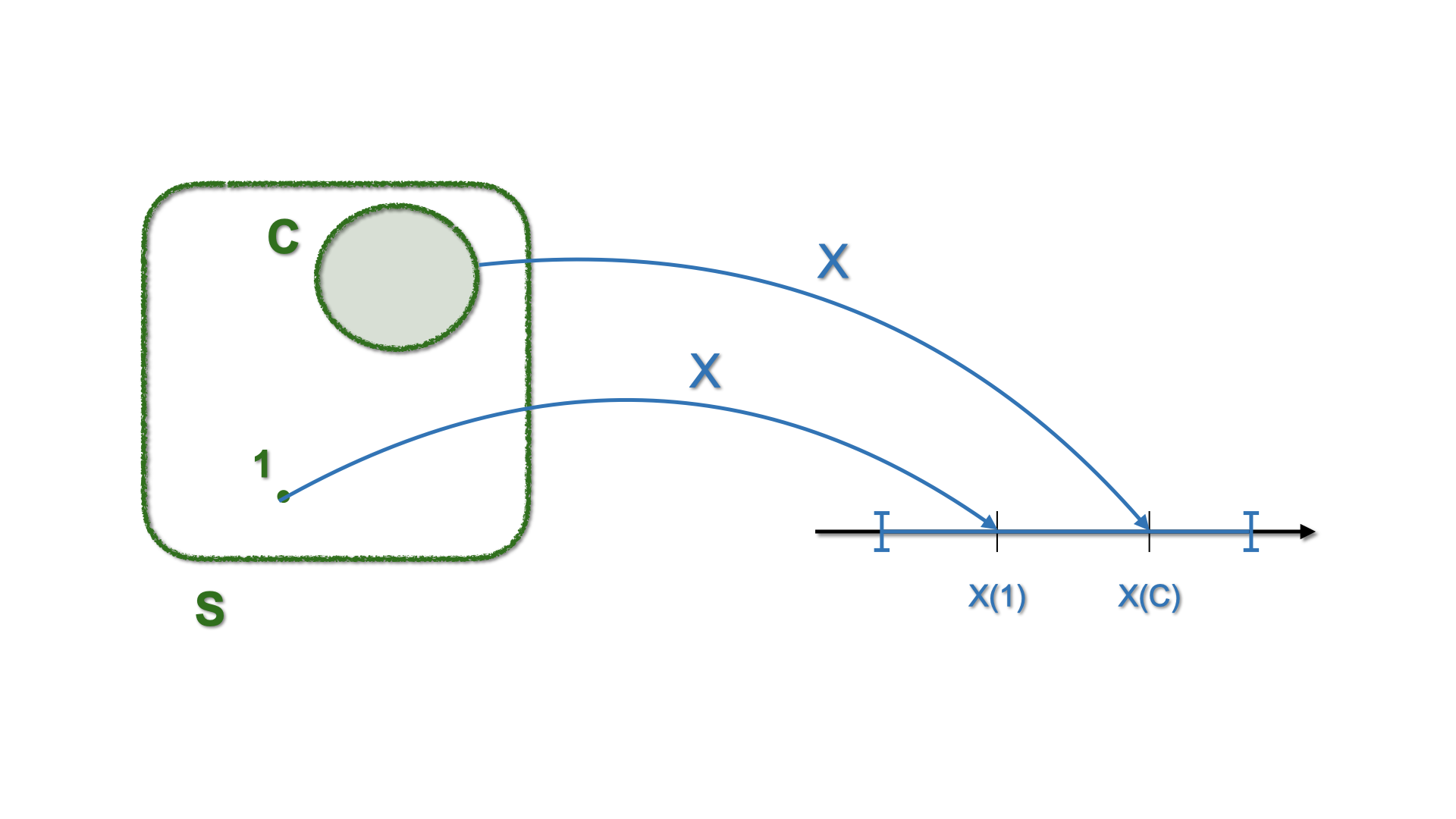
Figure 4.2: Schematic representation of mapping with a Random Variable

4.1.2 Example: from \(S\) to \(D\), via \(X(\cdot)\)

For the elements related to \(\color{green}S\) we have a probability \(\color{green}{Pr}\)

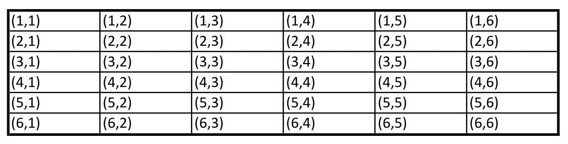
Now define \(X(\color{green}{s_{ij}})\) as the sum of the outcome \(i\) of the first die and the outcome \(j\) of the second die. Thus:

\[\begin{eqnarray*} X(\color{green}{s_{ij}})= X(i,j)= i+j, & \text{ for } & i=1,...,6, \text{ and } j=1,...,6 \end{eqnarray*}\]

In this notation \(\color{green}{s_{ij}=(i,j)}\) and \(\color{green}{s_{ij}\in S}\), each having probability \(1/36\).

Let us proceed to formalise this setting with a Random Variable and make the mapping explicit:

• \(X(\cdot)\) maps \(\color{green}{S}\) into \(\color{blue}D\). The (new) sample space \(\color{blue}{D}\) is given by: \[\begin{equation*} \color{blue}{D=\left\{2,3,4,5,6,7,8,9,10,11,12\right\}} \end{equation*}\] where, e.g., \(\color{blue}{2}\) is related to the pair \((1,1)\), \(\color{blue}{3}\) is related to the pairs \((1,2)\) and \((2,1)\), etc etc. So \(\color{blue}{D}\) is related the new \(\color{blue}{P}\)
• To each element (event) in \(\color{blue}{D}\) we can attach a probability, using the probability of the corresponding event(s) in \(S\). For instance, \[P(\color{blue}{2})=Pr(1,1)=1/36, \quad \text{or} \quad P(\color{blue}{3})=Pr(1,2)+Pr(2,1)=2/36.\]
• How about the \(P(\color{blue}{7})\)?
  \[\begin{equation*} P(\color{blue}7)=Pr(3,4)+Pr(2,5)+Pr(1,6)+Pr(4,3)+Pr(5,2)+Pr(6,1)=6/36. \end{equation*}\]
• The latter equality can also be re-written as \[P(\color{blue}7)=2(Pr(3,4)+Pr(2,5)+Pr(1,6))=6 \ Pr(3,4),\]

Let us formalise all these ideas:

For X to be a random variable it is required that for each event \(A\) consisting, if you will, of elements in \(D\): \[\begin{equation*} \color{blue}P\left( A\right) = \color{green} {Pr} ( \left\{ s\in S :X\left( s \right) \in A\right\}) \end{equation*}\] where \(\color{blue}{P}\) and \(\color{green}{Pr}\) stand for “probability” on \(\color{blue}{D}\) and on \(\color{green}{S}\), respectively, we assess the following properties (See Chapter 3):

• \(P \left( A\right) \geq 0\) %for all \(A\in \mathcal{B}_{D}\)
• \(\color{blue}P \left( D\right) =\color{green}Pr (\left\{ s\in S:X\left( s\right) \in D\right\}) =Pr \left( S\right) =1\)
• If \(A_{1},A_{2},A_{3}...\) is a sequence of events such that: \[A_{i}\cap A_{j}=\varnothing\] for all \(i\neq j\) then: \[\color{blue}P \left( \bigcup _{i=1}^{\infty }A_{i}\right) =\sum_{i=1}^{\infty } \color{blue} P\left( A_{i}\right).\]

In what follows we will be dropping the colors.

4.1.3 An Example from gambling

4.2 Discrete random variables

Discrete random variables are often associated with the process of counting. The previous example is a good illustration of that use. More generally, we can characterise the probability of any random variable as follows:

For a discrete random variable \(X\), any table listing all possible nonzero probabilities provides the entire probability distribution.

And the probability mass function \(p(a)\) of \(X\) is defined by: \[ p_a = p(a)= P(\{X=a \}), \] and this is positive for at most a countable number of values of \(a\). For instance, \(p_{1} = P(\left\{ X=x_1\right\})\), \(p_{2} = P(\left\{ X=x_2\right\})\), and so on.

That is, if \(X\) must assume one of the values \(x_1,x_2,...\), then \[\begin{eqnarray} p(x_i) \geq 0 & \text{for \ \ } i=1,2,... \\ p(x) = 0 & \text{otherwise.} \end{eqnarray}\]

Clearly, we must have \[ \sum_{i=1}^{\infty} p(x_i) = 1. \]

4.3 Cumulative Distribution Function

The cumulative distribution function (CDF) is a table listing the values that \(X\) can take, alongside the the cumulative probability, i.e. \[F_X(a) = P \left(\{ X\leq a\}\right)= \sum_{\text{all } x \leq a } p(x).\]

If the random variable \(X\) takes on values \(x_{1},x_{2},x_{3},\ldots .,x_{n}\) listed in increasing order \(x_{1}<x_{2}<x_{3}<\cdots <x_{n}\), the CDF is a step function, that it its value is constant in the intervals \((x_{i-1},x_i]\) and takes a step/jump of size \(p_i\) at each \(x_i\):

\(x_i\)	\(F_X(x_i)=P\left(\{ X\leq x_i\}\right)\)
\(x_{1}\)	\(p_{1}\)
\(x_{2}\)	\(p_{1}+p_{2}\)
\(x_{3}\)	\(p_{1}+p_{2}+p_{3}\)
\(\vdots\)	\(\vdots\)
\(x_{n}\)	\(p_{1}+p_{2}+\cdots +p_{n}=1\)

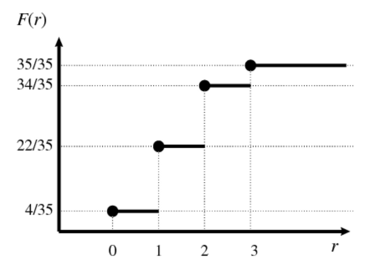
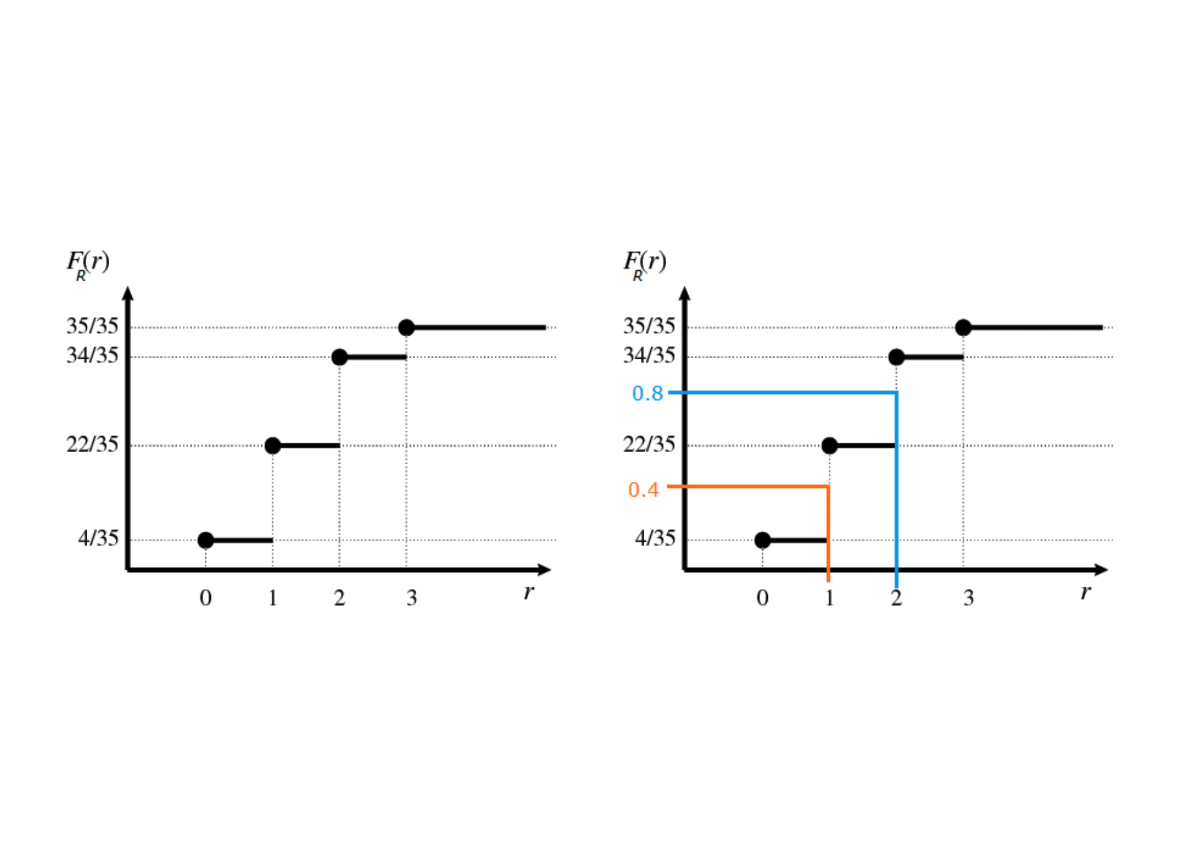
Figure 4.3: Step function

If we denote the random variable as \(R\), its realisations with \(r\) and the CDF evaluated in \(r\) as \(F_R(r)\), we can see graphically:

4.4 Distributional summaries for discrete random variables

In many applications, it is useful to describe some attributes or properties of the distribution of a Random Variable, for instance, to have an overview of how “central” a realisation is or how “spread” or variable the distribution really is. In this section, we will define two of these summaries:

• The Expectation, or Mean of the distribution is an indicator of “location.” It is defined as the mean of the realisations weighted by their probabilities, i.e.  \[\begin{equation*} E\left[ X\right] =p_{1}x_{1}+p_{2}x_{2}+\cdots + p_{n}x_{n} = \sum_{i=1}^{n} p_i x_i \end{equation*}\] Roughly speaking the mean represents the center of gravity of the distribution.

• The square root of the variance, or standard deviation, of the distribution is a measure of spread and is computed as the average squared distance between the observations with respect to the Expectation. \[\begin{eqnarray*} s.d\left( X\right) &=&\sqrt{Var\left( X\right) } \\ &=&\sqrt{p_{1}\left( x_{1}-E\left[ X\right] \right) ^{2}+p_{2}\left( x_{2}-E \left[ X\right] \right) ^{2}+\cdots + p_{n}\left( x_{n}-E\left[ X\right] \right) ^{2}} \end{eqnarray*}\] Roughly spread (or ‘variability’ or ‘dispersion’).

4.4.1 Properties

If \(X\) is a discrete random variable and \(a\) is any real number, then

• \(E\left[ \alpha X\right] =\alpha E\left[ X\right]\)
• \(E\left[ \alpha+X\right] =\alpha+E\left[ X\right]\)
• \(Var\left( \alpha X\right) =\alpha^{2}Var\left( X\right)\)
• \(Var\left( \alpha+X\right) =Var\left( X\right)\)

4.5 Dependence/Independence

4.5.1 More important properties

• If \(X\) and \(Y\) are two discrete random variables, then% \[\begin{equation*} E\left[ X+Y\right] =E\left[ X\right] +E\left[ Y\right] \end{equation*}\]

• If \(X\) and \(Y\) are also independent, then \[\begin{equation} Var\left( X+Y\right) =Var\left( X\right) +Var\left( Y\right) \label{Eq. Var} \end{equation}\]

4.5.2 More on expectations

Recall that the expectation of X was defined as \[\begin{equation*} E\left[ X\right] = \sum_{i=1}^{n} p_i x_i \end{equation*}\]

Now, suppose we are interested in a function \(m\) of the random variable \(X\), say \(m(X)\). We define \[\begin{equation*} E\left[ m\left( X\right) \right] =p_{1}m\left( x_{1}\right) +p_{2}m\left( x_{2}\right) +\cdots p_{n}m\left( x_{n}\right). \end{equation*}\]

Notice that the variance is a special case of expectation where, \[\begin{equation*} m(X)=(X-E\left[ X\right] )^{2}. \end{equation*}\] Indeed, \[\begin{equation*} Var\left( X\right) =E\left[ (X-E\left[ X\right] )^{2}\right]. \end{equation*}\]

4.6 Some discrete distributions of interest

• Discrete Uniform
• Bernoulli
• Binomial
• Poisson
• Hypergeometric
• Negative binomial

Their main characteristic is that the probability \(P\left(\left\{ X=x_i\right\}\right)\) is given by an appropriate mathematical formula: i.e.  \[p_{i}=P\left(\left\{ X=x_i\right\}\right)=h(x_{i})\] for a suitably specified function \(h(\cdot)\).

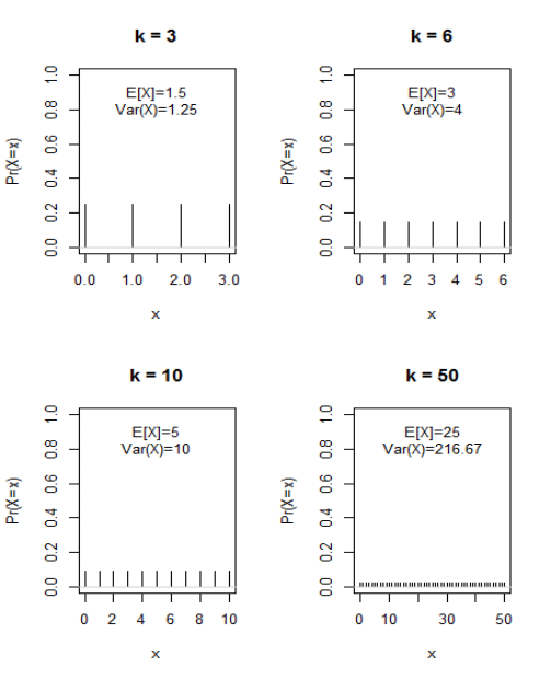
4.6.1 Discrete uniform distribution

4.6.1.1 Expectation

• The expected value of \(X\) is \[\begin{eqnarray*} E\left[ X\right] &=& x_1 p_1 + ... + x_k p_k\\ &=& 0\cdot \frac{1}{\left( k+1\right) }+1\cdot \frac{1}{% \left( k+1\right) }+\cdots +k\cdot \frac{1}{\left( k+1\right) } \\ &=&\frac{1}{\left( k+1\right) }\cdot\left( 0+1+\cdots +k\right) \\ &=&\frac{1}{\left( k+1\right) }\cdot \frac{k\left( k+1\right) }{2} \\ &=&\frac{k}{2}. \end{eqnarray*}\]

E.g. when \(k=6\), then \(X\) can take on one of the seven distinct values \(x=0,1,2,3,4,5,6,\) each with equal probability \(\frac{1}{7}\), but the expected value of \(X\) is equal to \(3\), which is one of the possible outcomes!!!

4.6.1.2 Variance

• The variance of \(X\) – we will be denoting it as \(Var(X)\) – is% \[\begin{eqnarray*} Var\left( X\right) &=&\left( 0-\frac{k}{2}\right) ^{2}\cdot \frac{1}{\left( k+1\right) }+\left( 1-\frac{k}{2}\right) ^{2}\cdot \frac{1}{\left( k+1\right) }+ \\ &&\cdots +\left( k-\frac{k}{2}\right) ^{2}\cdot \frac{1}{\left( k+1\right) } \\ &=&\frac{1}{\left( k+1\right) }\cdot\left\{ \left( 0-\frac{k}{2}\right) ^{2}+\left( 1-\frac{k}{2}\right) ^{2}+\cdots +\left( k-\frac{k}{2}\right) ^{2}\right\} \\ &=&\frac{1}{\left( k+1\right) }\cdot \frac{k\left( k+1\right) \left( k+2\right) }{12} \\ &=&\frac{k\left( k+2\right) }{12} \end{eqnarray*}\]

E.g. when \(k=6\), the variance of \(X\) is equal to \(4,\) and the standard deviation of \(X\) is equal to \(\sqrt{4}=2.\)

4.6.1.3 Illustrations

4.6.2 Bernoulli Trials

Often we write the probability mass function (PMF) as:

\[\begin{equation*} P(\left\{ X=x\right\})=p^{x}\left( 1-p\right) ^{1-x}, \quad \text{ for }x=0,1 \end{equation*}\]

A Bernoulli trial represents the most primitive form of all random variables. It derives from a random experiment having only two possible mutually exclusive outcomes. These are often labelled Success and Failure and

• Success occurs with probability \(p\)
• Failure occurs with probability \(1-p\).

4.6.2.1 Expectation

\[\begin{eqnarray*} E\left[ X\right] &=&1 \cdot p+0 \cdot (1-p) \\ &=&p \end{eqnarray*}\]

4.6.2.2 Variance

\[\begin{eqnarray*} Var\left( X\right) &=&\left( 1-p\right) ^{2} \cdot p+\left( 0-p\right) ^{2} \cdot \left( 1-p\right) \\ &=&p\left( 1-p\right). \end{eqnarray*}\]

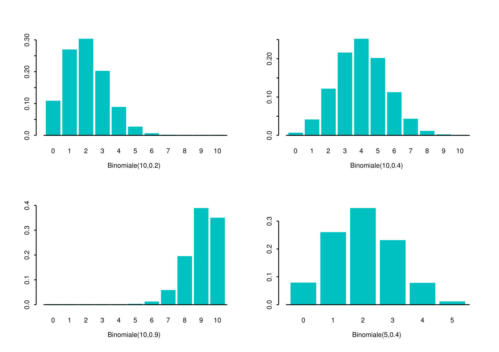
4.6.3 The Binomial Distribution

You might recall from Chapter 1 that Combinations are defined as: \[\begin{equation*} {n \choose k} =\frac{n!}{k!\left( n-k\right) !}=C^{k}_{n} \end{equation*}\] and, for \(n \geq k\), we say ``\(n\) choose \(k\)’’.

The binomial coefficient \(n \choose k\) represents the number of possible combinations of \(n\) objects taken \(k\) at a time, without regard of the order. Thus, \(C^{k}_{n}\) represents the number of different groups of size \(k\) that could be selected from a set of \(n\) objects when the order of selection is not relevant.

So, “What is the interpretation of the formula?”

• The first factor \[{n \choose k} =\frac{n!}{x!\left( n-x\right)!}\] is the number of different combinations of individual “successes” and “failures” in \(n\) (Bernoulli) trials that result in a sequence containing a total of \(x\) ‘successes’ and \(n-x\) “failures.”
• The second factor \[p^{x}\left( 1-p\right) ^{n-x}\] is the probability associated with any one sequence of \(x\) ‘successes’ and \((n-x)\) `failures’.

4.6.3.1 Expectation

\[\begin{eqnarray*} E\left[ X\right] &=&\sum_{x=0}^{n}x\Pr \left\{ X=x\right\} \\ &=&\sum_{x=0}^{n}x {n\choose k} p^{x}\left(1-p\right) ^{n-x} = np \end{eqnarray*}\]

4.6.3.2 Variance

\[\begin{eqnarray*} Var\left( X\right) &=&\sum_{x=0}^{n}\left( x-np\right) ^{2} P (\left\{ X=x\right\}) \\ &=&np\left( 1-p\right) \end{eqnarray*}\]

4.6.3.3 Illustrations

The visualisation shows some similiarities to the Discrete Uniform but some values seem more probable than others. Moreover, the shape of the distribution seems to vary according to the values of \(n\) and \(p\), i.e the parameters of the distribution.

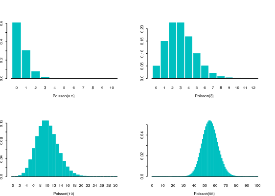
4.6.4 Poisson Distribution

The Eq. () defines a genuine probability mass function, since \(p(x) \geq 0\) and

\[\begin{eqnarray} \sum_{x=0}^{\infty} p(x) &=& \sum_{x=0}^{\infty} \frac{\lambda ^{x}e^{-\lambda }}{x!} \\ & = & e^{-\lambda } \sum_{x=0}^{\infty} \frac{\lambda ^{x}}{x!} \\ & = & e^{-\lambda } e^{\lambda } = 1 \quad \text{(see Intro Lecture).} \end{eqnarray}\]

Moreover, for a given value of $$ also the CDF can be easily defined. E.g.

\[\begin{equation*} F_X(2)=\Pr \left( \{X\leq 2\}\right) =e^{-\lambda }+\lambda e^{-\lambda }+\frac{\lambda ^{2}e^{-\lambda }}{2}, \end{equation*}\]

and the Expected value and Variance for Poisson distribution (see tutorial) can be obtained by ‘’sum algebra’’ (and/or some algebra)

\[\begin{eqnarray*} E\left[ X\right] &=&\lambda \\ Var\left( X\right) &=&\lambda. \end{eqnarray*}\]

4.6.4.1 Illustrations

… same barplot as in slide 30, just a bit fancier…

4.6.4.2 Link to Binomial

Let us consider \(X \sim B(x,n,p)\), where \(n\) is large, \(p\) is small, and the product \(np\) is appreciable. Setting, \(\lambda=np\), we then have that, for the Binomial probability as in Eq.(), it is a good approximation to write: \[ p(k) = P(\{X=k\}) \approx \frac{\lambda^k}{k!} e^{-\lambda}. \] To see this, remember that
\[ \lim_{n\rightarrow\infty} \left( 1- \frac{\lambda}{n} \right)^n = e^{-\lambda}. \] Then, let us consider that in our setting, we have \(p=\lambda/n\). From the formula of the binomial probability mass function we have: \[ p(0) = (1-p)^{n}=\left( 1- \frac{\lambda}{n} \right)^{n} \approx e^{-\lambda}, \quad \text{\ as \ \ } n\rightarrow\infty. \]

Moreover, it is easily found that

\[\begin{eqnarray} \frac{p(k)}{p(k-1)} &=& \frac{np-(k-1)p}{k(1-p)} \approx \frac{\lambda}{k}, \quad \text{\ as \ \ } n\rightarrow\infty. \end{eqnarray}\]

Therefore, we have

\[\begin{eqnarray} p(1) &\approx& \frac{\lambda}{1!}p(0) \approx \lambda e^{-\lambda} \\ p(2) &\approx& \frac{\lambda}{2!}p(1) \approx \frac{\lambda^2}{2} e^{-\lambda} \\ \dotsm & \dotsm & \dotsm \\ p(k) &\approx& \frac{\lambda}{k!}p(k-1) \approx \underbrace{\frac{\lambda^k}{k!} e^{-\lambda}}_{\text{\ see \ \ Eq. (\ref{Eq. Poisson}) }} \end{eqnarray}\]

thus, we remark that \(p(k)\) can be approximated by the probability mass function of a Poisson—which is easier to implement.

4.6.5 The Hypergeometric Distribution

Moreover,

\[\begin{eqnarray*} E\left[ X\right] &=&\frac{nk}{N} \\ Var\left( X\right) &=&\frac{nk\left( N-k\right) \left( N-n\right) }{% N^{2}\left( N-1\right) } \end{eqnarray*}\]

4.6.5.1 Illustrations

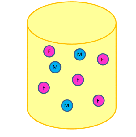
Consider each of the three participants being selected as a separate trial $$ there are \(n=3\) trials. Consider a woman being selected in a trial as a `success’ \ Then here \(N=8\), \(k=5\), \(n=3\), and \(x=2\), so that% \[\begin{eqnarray*} \Pr (\left\{ X=2\right\}) &=&\frac{\left( \begin{array}{c} 5 \\ 2% \end{array}% \right) \left( \begin{array}{c} 8-5 \\ 3-2% \end{array}% \right) }{\left( \begin{array}{c} 8 \\ 3% \end{array}% \right) } \\ && \\ &=&\frac{\frac{5!}{2!3!}\frac{3!}{1!2!}}{\frac{8!}{5!3!}} \\ && \\ &=&0.53571 \end{eqnarray*}\]

4.6.6 The Negative Binomial Distribution

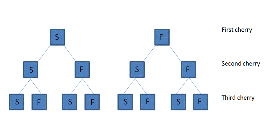
Let us consider a random experiment consisting of a series of trials, having the following properties

• Only two mutually exclusive outcomes are possible in each trial: success' (S) andfailure’ (F)

• The outcomes in the series of trials constitute independent events

• The probability of success \(p\) in each trial is constant from trial to trial

What is the probability of having exactly \(y\) F’s before the \(r^{th}\) S?

Equivalently: What is the probability that in a sequence of \(y+r\) (Bernoulli) trials the last trial yields the \(r^{th}\) S?

The mean and variance for \(X\) are, respectively,%

\[\begin{eqnarray*} E\left[ X\right] &=&\frac{r}{p} \\ Var\left( X\right) &=&\frac{r\left( 1-p\right) }{p^{2}} \end{eqnarray*}\]

4.6.7 Illustrations

4.6.8 The Geometric Distribution

The corresponding mean and variance for \(X\) are, respectively,

\[\begin{eqnarray*} E\left[ X\right] &=&\frac{ 1 }{p} \\ Var\left( X\right) &=&\frac{\left( 1-p\right) }{p^{2}} \end{eqnarray*}\]

More generally, for a geometric random variable we have:

\[P(\{X \geq k \}) = (1-p)^{k-1}\]

Thus, in the example we have \(P( \{X \geq 6 \}) = (1-0.03)^{6-1}\approx 0.8587\)

\[\begin{eqnarray} P(\{X \leq 5\}) = 1-P( \{X \geq 6 \}) \approx 1- 0.8587 \approx 0.1412. \end{eqnarray}\]