11 Power: You either have it or you don’t
The most frequently asked question by my students is: How much data do I have to collect? My answer is always the same: ‘It depends’. From a student’s perspective, this must be one of the most frustrating answers. Usually, I follow this sentence up with something more helpful to guide students on their way. For example, there is a way to determine how large your sample has to be to detect specific relationships reliably. This procedure is called power analysis.
While power analysis can be performed before and after data collection, it seems rather pointless to do it afterwards when collecting more data is not only challenging but sometimes impossible. Thus, my explanations in this chapter will primarily focus on the question: How much data is enough to detect relationships between variables reliably.
Power analysis is something that applies to all kinds of tests, such as correlations (Chapter 10), group comparisons (Chapter 12) and regressions (Chapter 13). Therefore, it is important to know about it. There is nothing worse than presenting a model or result that is utterly ‘underpowered’, i.e. the sample is not large enough to detect the desired relationship between variables reliably. In anticipation of your question about whether your analysis can be ‘overpowered’, the answer is ‘yes’. Usually, there are no particular statistical concerns of having an overpowered analysis - more power to you (#pun-intended). However, collecting too much data can be an ethical concern. If we think of time as a scarce resource, we should not collect more data than we need. Participants’ time is valuable and being economic during data collection is essential. We do not have to bother more people with our research than necessary because not everyone is as excited about your study as you are. Besides, if everyone conducts studies on many people, effects such as survey fatigue can set in, making it more difficult for others to carry out their research. Thus, being mindful of the required sample size is always important - I mean: essential.
11.1 Ingredients to achieve the power you deserve
We already know that sample size matters, for example, to assume normality when there is none in your sample (see Central Limit Theorem in Chapter 9.3). Also, we should not mistakenly assume that a relationship exists where there is none and vice versa. I am referring to so-called Type I and Type II errors (see Table 11.1).
| Error | Meaning |
|---|---|
| Type I |
|
| Type II |
|
Power analysis aims to help us avoid type II errors and is defined as the opposite of it, i.e. \(1 - \beta\), i.e. a ‘true positive’. To perform such a power analysis, we need at least three of the following four ingredients:
the power level we want to achieve, i.e. the probability that we find a ‘true positive’,
the expected effect size (\(r\)) we hope to find,
the significance level we set for our test, i.e. how strict we are about deciding when a relationship is significant, and
the sample size.
As I mentioned earlier, it makes more sense to use a power analysis to determine the sample size. However, in the unfortunate event that you forgot to do so, at least you can find out whether your results are underpowered by providing the sample size you collected. If you find that your study is underpowered, you are in serious trouble and dire need of more participants.
11.2 Computing power
So, how exactly can we compute the right sample size, and how do we find all the numbers for these ingredients without empirical data at our disposal? First, we need a function that can compute it because computing a power analysis manually is quite challenging. The package pwr was developed to do precisely that for different kinds of statistical tests. Table 11.2 provides an overview of functions needed to perform power analysis for various tests covered in this book.
| Statistical method | Chapter | function in pwr |
|---|---|---|
| Correlation | Chapter 10 | pwr.r.test() |
| T-test | Chapter 12 |
|
| ANOVA | Chapter 12.3 | pwr.anova.test() |
| Chi-squared test | Chapter 12.4 | pwr.chisq.test() |
| Linear regression | Chapter 13 | pwr.f2.test() |
Since all functions work essentially the same, I will provide an example of last chapter’s correlation analysis. You likely remember that we looked at whether the number of votes a movie receives on IMDb can predict its earnings. Below is the partial correlation that revealed a relationship in our sample based on the top 250 movies. This is just a sample, and it is not representative of all movies listed on IMDb because it only includes the best movies of all time. As of June 2021, IMDb offers information about 8 million movie titles.
imdb_top_250 %>%
  select(votes, gross_in_m, year) %>%
  correlation(partial = TRUE)
#> Registered S3 methods overwritten by 'parameters':
#>   method                           from
#>   as.double.parameters_kurtosis    datawizard
#>   as.double.parameters_skewness    datawizard
#>   as.double.parameters_smoothness  datawizard
#>   as.numeric.parameters_kurtosis   datawizard
#>   as.numeric.parameters_skewness   datawizard
#>   as.numeric.parameters_smoothness datawizard
#>   print.parameters_distribution    datawizard
#>   print.parameters_kurtosis        datawizard
#>   print.parameters_skewness        datawizard
#>   summary.parameters_kurtosis      datawizard
#>   summary.parameters_skewness      datawizard
#> # Correlation Matrix (pearson-method)
#>
#> Parameter1 | Parameter2 |    r |       95% CI | t(213) |         p
#> ------------------------------------------------------------------
#> votes      | gross_in_m | 0.48 | [0.37, 0.58] |   7.98 | < .001***
#> votes      |       year | 0.28 | [0.16, 0.40] |   4.31 | < .001***
#> gross_in_m |       year | 0.16 | [0.03, 0.29] |   2.43 | 0.016*
#>
#> p-value adjustment method: Holm (1979)
#> Observations: 215
Let’s define our ingredients to compute the ideal sample size for our correlation:
Power: J. Cohen (1988) suggests that an acceptable rate of type II error is \(\beta = 0.2\) (i.e. 20%). Thus, we can define the expected power level as \(power = 1 - 0.2 = 0.8\).
Significance level (i.e. \(\alpha\)): We can apply the traditional cut-off point of
0.05(see also Chapter 10.3).Effect size: This value is the most difficult to judge but substantially affects your sample size. It is easier to detect big effects than smaller effects. Therefore, the smaller our
r, the bigger our sample size has to be. We know from our correlation that the effect size is0.48, but what can you do to estimate your effect size if you do not have data available. Unfortunately, the only way to acquire an effect size is to either use simulated data or, as most frequently is the case, we need to refer to reference studies that looked at similar phenomena. I would always aim for slightly smaller effect sizes than expected, which means I need a larger sample. If the effect is bigger than expected, we will not find ourselves with an underpowered result. Thus, for our example, let’s assume we expected \(r = 0.4\).
All there is left to do is insert these parameters into our function pwr.r.test().
pwr::pwr.r.test(r = 0.4,
                sig.level = 0.05,
                power = 0.8)
#>
#>      approximate correlation power calculation (arctangh transformation)
#>
#>               n = 45.91614
#>               r = 0.4
#>       sig.level = 0.05
#>           power = 0.8
#>     alternative = two.sided
To find the effect we are looking for, we only need 46 movies (we always round up!), and our dataset contains 250 observations. Thus, we are considerably overpowered for this type of analysis. What if we change the parameters slightly and expect \(r = 0.3\) and increase increase our threshold of accepting a true relationship, i.e. \(p = 0.01\)?
pwr::pwr.r.test(r = 0.3,
                sig.level = 0.01,
                power = 0.8)
#>
#>      approximate correlation power calculation (arctangh transformation)
#>
#>               n = 124.405
#>               r = 0.3
#>       sig.level = 0.01
#>           power = 0.8
#>     alternative = two.sided
The results show that if we are stricter with our significance level and look for a smaller effect, we need about three times more movies in our sample, i.e. at least 125.
Given that we already know our sample size, we could also use this function to determine the power of our result ex-post. This time we need to provide the sample size n and we will not specify power.
pwr::pwr.r.test(n = 215,
                r = 0.48,
                sig.level = 0.01)
#>
#>      approximate correlation power calculation (arctangh transformation)
#>
#>               n = 215
#>               r = 0.48
#>       sig.level = 0.01
#>           power = 0.9999998
#>     alternative = two.sided
The results reveal that our power level is equivalent to cosmic entities, i.e. extremely powerful. In other words, we would not have needed a sample this large to find this genuine relationship.
11.3 Plotting power
Lastly, I want to show you how to create a plot that reveals the different sample sizes needed to achieve \(power = 0.8\). It visually demonstrates how much more data we need depending on the effect size. For the plot, I set a power level (i.e. 0.8) and significance levels of 0.01 and 0.05. I only varied effect sizes to see the required sample size.
# Create a tibble with effect size r
power_df <- tibble(r = seq(from = 0.1,
                           to =  0.9,
                           by = 0.01))

# We need to compute the sample size for each effect size level
power_df <-
  power_df %>%
  rowwise() %>%
  mutate(n_0.01 =
           broom::tidy(pwr::pwr.r.test(r = r,
                                       sig.level = 0.01,
                                       power = 0.8)) %>%
           first(),
         n_0.05 =
           broom::tidy(pwr::pwr.r.test(r = r,
                                       sig.level = 0.05,
                                       power = 0.8)) %>%
           first())

glimpse(power_df)
#> Rows: 81
#> Columns: 3
#> Rowwise:
#> $ r      <dbl> 0.10, 0.11, 0.12, 0.13, 0.14, 0.15, 0.16, 0.17, 0.18, 0.19, 0.2…
#> $ n_0.01 <dbl> 1162.56417, 959.87066, 805.70532, 685.72827, 590.52987, 513.728…
#> $ n_0.05 <dbl> 781.75156, 645.53169, 541.92525, 461.29509, 397.31753, 345.7036…
# Plot the effect sizes against the sample size
power_df %>%
ggplot() +
# The line for p = 0.01
geom_line(aes(x = r,
y = n_0.01,
col = "p = 0.01")) +
# The line for p = 0.05
geom_line(aes(x = r,
y = n_0.05,
col = "p = 0.05")) +
# Add nice labels
labs(col = "Sig. levels",
x = "r",
y = "n")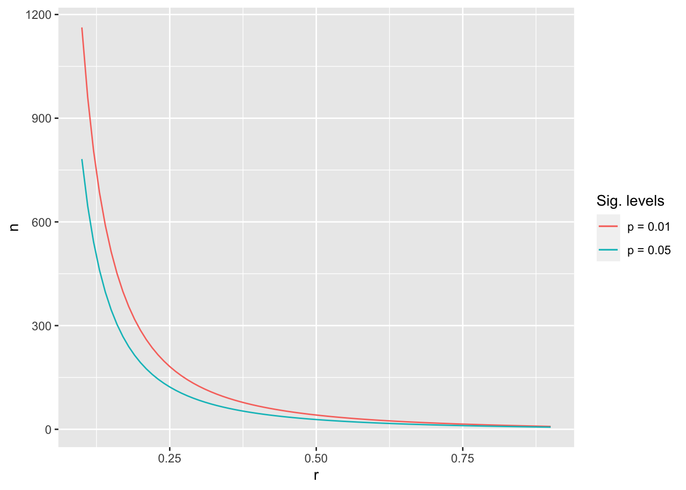
The results reveal that the relationship between n and r is logarithmic and not linear. Thus, the smaller the effect size, the more difficult it is to reach reliable results.
The R code to produce this plot features broom::tidy() and first(). The function tidy() from the broom package converts the result from pwr.r.test() from a list to a tibble, and the function first() picks the first entry in this tibble, i.e. our sample sizes. Don’t worry if this is confusing at this stage. We will return to tidy() in later chapters, where its use becomes more apparent.
11.4 Concluding remarks about power analysis
Conducting a power analysis is fairly straightforward for the techniques we cover in this book. Therefore there is no excuse to skip this step in your research. The challenging part for conducting a power analysis in advance is the definition of your effect size. If you feel you cannot commit to a single effect size, specify a range, e.g. \(0.3 < effect size < 0.5\). This will provide you with a range for your sample size.
For statistical tests like group comparisons (Chapter 12) and regressions (Chapter 13), the number of groups or variables also plays an important role. Usually, the more groups/variables are included in a test/model, the larger the sample has to be.
As mentioned earlier, it is not wrong to collect slightly more data, but you need to be cautious not to waste ‘resources’. In other fields, like medical studies, it is absolutely critical to know how many patients should be given a drug to test its effectiveness. It would be unethical to administer a new drug to 300 people when 50 would be enough. This is especially true if the drug turns out to have an undesirable side effect. In Social Sciences, we are not often confronted with health-threatening experiments or studies. Still, being mindful of how research impacts others is essential. A power analysis can help to determine how you can carry out a reliable study without affecting others unnecessarily.