3 Bayesian vs. frequentist probability
In the previous module, we looked at the reasoning behind frequentist inference. In this module, we will introduce Bayesian inference, and explore how frequentist and Bayesian approaches differ.
3.1 Relative frequency
3.1.1 Quick recap
A quick summary of the main points from the previous module:
The frequentist approach treats probabilities as relative frequencies. If we say that the probability of rolling a 5 on a fair die is \(\frac{1}{6}\), we mean that, if the die were rolled an infinite number of times, \(\frac{1}{6}^{th}\) of all rolls would be a 5. More practically, if we roll the die a large (but non-infinite) number of times, we will predict (or “expect”) \(\frac{1}{6}^{th}\) of our rolls to land on 5.
If we say the probability of getting a test statistic at least as large as \(z=\pm 1.96\) under a null hypothesis is \(0.05\), what we mean is that, if could take an infinite number of samples from the same population and the null hypothesis is true, then we will get \(𝑧\geq|1.96|\) 1 out of every 20 times.
If we say that a \(95\%\) CI has \(95\%\) coverage probability for a parameter \(\theta\), what we mean is that, if we could take an infinite number of samples from the same population, our method would produce an interval that contains \(\theta\) in 19 out of every 20 samples.
Frequentist probability is sometimes thought of as “physical” probability, because it quantifies rates of outcomes in physical processes that we are willing to characterize as random.
3.1.2 What frequentism does not allow
Frequentist probabilities can only be assigned to random variables.
Data are considered random (“we took a random sample of…”). Statistics are calculated from data, and so statistics are considered random variables. We can make probability statements about the values that statistics will take on.
Hypotheses are not random. Parameters are not random. “The truth” is not random. Frequentist probabilities cannot be assigned to these.
This might explain why frequentist interpretations sometimes feel strange: we must always be careful to direct our probability statements at statistics or data, and not at hypotheses or parameters.
Examples:
We cannot talk about “the probability that the null hypothesis is true”, because the truth value of the null hypothesis is not random. The null is either true or false. Just because we don’t know whether it is true or false does not make whether it is true or false a random variable. Instead, we talk about the probability of getting some kind of statistical result if the null is true, or if the null is false.
We cannot talk about the probability that a parameter’s value falls inside a particular confidence interval. The parameter’s value is not a random variable. And once data have been collected, the “random” part is over and the confidence interval’s endpoints are known. There is now nothing random going on. Either the parameter value is inside the interval or it is outside the interval. The fact that we don’t know the parameter’s value does not make its value a random variable. Instead, we talk about the probability that a new random sample, not yet collected, would produce a confidence interval that contains the unknown parameter value.
3.2 Degrees of belief
The Bayesian approach treats probability as quantifying a rational degree of belief. This approach does not require that variables be “random” in order to make probability statements about their values. It does not require that probabilities be thought of as long run relative frequencies17.
Here are some probabilities that do not make sense from the frequentist perspective, but make perfect sense from the Bayesian perspective:
The probability that a hypothesis is true.
The probability that \(\mu_1-\mu_2\) falls inside a 95% confidence interval that we just computed.
The probability that a fever you had last week was caused by the influenza virus
The probability that the person calling you from an unknown telephone number wants to sell you something.
The probability that an election was rigged.
The probability that a witness testifying in court is lying about how they first met the defendant.
These probabilities do not refer to frequencies18. They refer to how much belief we are willing to apply to an assertion.
The mathematics of probabililty work the same in the Bayesian approach as they do in the frequentist approach. Bayesians and frequentists sometimes choose to use different mathematical tools, but there is no disagreement on the fundamental laws of mathematical probability. The disagreement is on what statistical methods to use, and how to interpret probabilistic results.
3.2.1 Bayes doesn’t need randomness
The Bayesian approach does not require anything to be random. Pierre-Simon Laplace, who did work on mathematical probability and who used the Bayesian approach to inference, believed that the universe was deterministic:
We may regard the present state of the universe as the effect of its past and the cause of its future. An intellect which at a certain moment would know all forces that set nature in motion, and all positions of all items of which nature is composed, if this intellect were also vast enough to submit these data to analysis, it would embrace in a single formula the movements of the greatest bodies of the universe and those of the tiniest atom; for such an intellect nothing would be uncertain and the future just like the past would be present before its eyes.
There is no contradiction here between determinism and using probability, as probability is simply quantifying our belief, or our information, or our ignorance.
3.3 Priors and updating
Does this all sound wonderful and amazing? There’s one more important element: priors.
“Priors” refer to beliefs held prior to your data analysis, or information known before you data analysis. They take the form of probabilities.
- A prior can be a single probability of some statement being true. Examples: the prior probability that a null hypothesis is true; the prior probability that a witness in court is lying.
- A prior can be a probability distribution, which assigns probabilities to all the values that a variable might take on. Example: the prior distribution for the effectiveness of a Facebook ad on ticket sales for concerts, defined as the % change in tickets sold when comparing concerts that are advertised on Facebook to those that are not. Such a prior distribution might look like this:
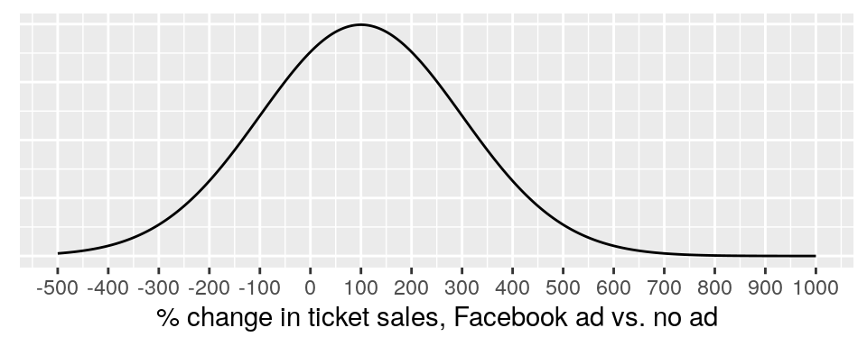
This is showing a prior probability distribution for \(P(effectiveness)\), defined as \(Normal(\mu=100,sd=200)\) This is a fairly weak prior distribution: it is centered on 100% (or a doubling of sales), but it has a standard deviation of 200, thus allowing some prior probability for unlikely values (300% decrease; 600% increase).
A stronger prior might look like this:
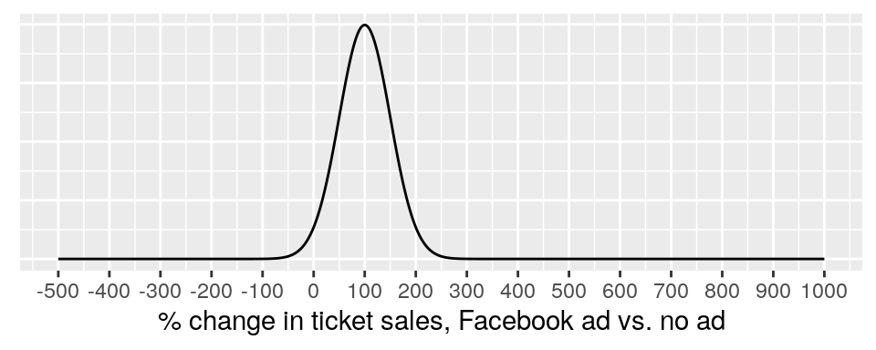
This is a “stronger” prior distribution than before, because it is effectively ruling out the extreme possibilities for changes in ticket sales.
We might also choose a distribution other than normal, since it seems unlikely that the ad will reduce sales. Maybe we find a distribution that gives a long right tail, giving some probability that the ad will have a huge positive effect on sales, but also a short left tail, giving very little probability to the ad being counterproductive to a large degree.
A prior is effectively a probability “starting point” that you set before seeing data. The data are then combined with the prior to “update” the beliefs or information contained in the original prior, giving a “posterior”.
Priors are essential to Bayesian inference. If we want to make a probability statement about a theory or a hypothesis using data, we need to establish our starting point.
Now might be a good time to take a look at “Bayes’ Rule”:
\[ P(B|A)=\frac{P(A|B)P(B)}{P(A)} \] In Bayesian statistics, we are typically drawing inference on parameters, using data. Call the parameters \(\boldsymbol{\theta}\) and the data \(\textbf{X}\):
\[ P(\boldsymbol{\theta}|\textbf{X}) =\frac{P(\textbf{X}|\boldsymbol{\theta})P(\boldsymbol{\theta})}{P(\textbf{X})} \] Where
- \(P(\boldsymbol{\theta}|\textbf{X})\) is the posterior probability distribution of the parameter
- \(P(\textbf{X}|\boldsymbol{\theta})\) is the likelihood of the data, given the parameters
- \(P(\boldsymbol{\theta})\) is the prior probability distribution of theta
- \(P(\textbf{X})\) is the total probability of the data
3.3.1 Example: screening test
Suppose that a routine COVID-19 screening test returns a positive result. And, suppose the test has a 2% false positive rate, meaning that if you don’t have COVID-19, there is only a 2 in 100 chance of testing positive. Does this mean that there is a 98% chance that you do have COVID-19?
No. The chance that a person without COVID-19 tests positive is not the same thing as the chance that a person who tests positive has COVID-19:
\[ P(test\ positive\ |\ no\ COVID) \neq P(no\ COVID\ |\ test\ positive) \] The only way to determine \(P(no\ COVID\ |\ test\ positive)\) from \(P(test\ positive\ |\ no\ COVID)\) is to use Bayes’ rule:
\[ P(no\ COVID\ |\ test\ positive)=\frac{P(test\ positive\ |\ no\ COVID)P(no\ COVID)}{P(test\ positive)} \] \(P(no\ COVID)\) is the prior probability of not having COVID-19. How do we decide this value?
- We may use current estimates for the % of the population who have COVID-19 at any given time.
- We may consider “daily life” factors that vary by individual, such as how much time is spent indoors with other people for long periods of time, or whether there’s been a known COVID-19 exposure
- We may consider whether a person has been infected previously.
- We may consider whether a person has been vaccinated.
There is no “objective” way to decide a prior. It is necessarily subjective. Hopefully, it is reasonably well justified.
\(P(test\ positive)\) is the probability that anyone will test positive, whether they have COVID-19 or not. It is the “total probability” of a positive test result.
Let’s suppose that the prior probability of not having COVID-19 is 96%, and that the probability of anyone testing positive is 5%. Then, we have:
\[ \begin{split} P(no\ COVID\ |\ test\ positive)&=\frac{P(test\ positive\ |\ no\ COVID)P(no\ COVID)}{P(test\ positive)} \\ \\ &= \frac{0.02*0.96}{0.05}=0.384 \end{split} \] So, in our hypothetical scenario, we have tested positive using a test that has only a 2% probability of a false positive. And, there is a 38.4% probability that our positive test was a false positive.
3.3.2 Example: evidence for a crime
Suppose there is a hit and run car accident, where someone causes an accident and then drives off. The victim didn’t see the driver, but did see that the other vehicle was a red truck. Suppose also that 4% of all people drive red trucks.
The police get a tip that someone was overheard at a bar bragging about getting away with running into someone and then driving off. A police officer goes to this person’s house and lo and behold! There’s a red truck in the driveway. Since only 4% of all people drive red trucks, the officer concludes that there is a 96% chance that this person is guilty.
This reasoning is invalid, and common enough to have its own name: the “prosecutor’s fallacy”, or the “base rate fallacy”. The key problem here is the same one we saw in the last example:
\[ P(not\ guilty\ |\ red\ truck) \neq P(red\ truck\ |\ not\ guilty) \] The missing piece of information is the prior probability of the suspect being guilty prior to seeing the evidence of the red truck. Again, if we are going to assign a probability to a hypothesis using data, we need a starting point!
Let’s say that, based on the police tip, we give this suspect a 20% chance of being guilty prior to us seeing the red truck. Let’s also allow for a 10% probability that the suspect is keeping the red truck somewhere else, out of fear of being caught. Using Bayes’s rule:
\[ \begin{split} P(not\ guilty\ |\ red\ truck)\ &= \frac{P(red\ truck\ |\ not\ guilty)P(not\ guilty)}{P(red\ truck)}\\ \\ \ &=\ \frac{P(red\ truck\ |\ not\ guilty)P(not\ guilty)}{P(red\ truck\ |\ not\ guilty)P(not\ guilty)+P(red\ truck\ |\ guilty)P(guilty)} \\ \\ \ &=\frac{(0.04)(0.8)}{(0.04)(0.8)+(0.90)(0.2)} \\ \\ \ &=0.1509\approx 15\% \end{split} \] We might now be concerned that our posterior probability is heavily influenced by our priors: \(P(not\ guilty)\) and \(P(red\ truck\ |\ guilty)\). A good practice is to try out different values and see how much effect this has on the posterior.
3.3.3 Example: \(P(H_0\ true)\)
We noted in the last chapter that, under frequentist inference, it doesn’t make sense to talk about the probability that a null hypothesis is true. This is because the truth status of the null hypothesis is not a random variable.
For Bayesian inference, this is not a problem. If we want the probability of the null hypothesis being true, given our data, we can use Bayes’ rule. And this mean that we must state a prior for \(P(H_0\ true)\)!
\[ \begin{split} P(H_0\ true\ |\ reject\ H_0)&=\frac{P(reject\ H_0\ |\ H_0\ true)P(H_0\ true)}{P(reject\ H_0)} \\ \\ &=\frac{P(reject\ H_0\ |\ H_0\ true)P(H_0\ true)}{P(reject\ H_0\ |\ H_0\ true)P(H_0\ true)+P(reject\ H_0\ |\ H_0\ false)P(H_0\ false)} \\ \\&= \frac{P(Type\ I\ error)P(H_0\ true)}{P(Type\ I\ error)P(H_0\ true)+Power\cdot P(H_0\ false)} \end{split} \] Now, suppose we collect some data and we reject \(H_0\). We are now wondering how likely it is that \(H_0\) is actually true. To do this, we need:
- A prior probability of \(H_0\) being true
- An assumed power for the test, where power is \(P(reject\ H_0\ |\ H_0\ is\ false)\)
Example 1:
\Let’s say we choose \(P(H_0)=0.5\) and \(Power=0.8\), and we rejected \(H_0\) at the \(\alpha=0.05\) level of significance, implying \(P(Type\ I\ error)=0.05\). Plugging these values into Bayes’ rule:
\[ \begin{split} &\frac{P(Type\ I\ error)P(H_0\ true)}{P(Type\ I\ error)P(H_0\ true)+Power\cdot P(H_0\ false)} \\ \\&=\frac{0.05\cdot0.5}{0.05\cdot0.5+0.8\cdot0.5}=\frac{0.025}{0.025+0.4}=0.0588 \end{split} \] Oh, hooray! The probability that the null hypothesis is true turns out to be very similar to 0.05, the Type I error rate. So, in this case, \(P(H_0\ true\ |\ reject\ H_0) \approx P(reject\ H_0\ |\ H_0\ true)\). Maybe this always happens!?!?!?!?!?19
Example 2 \Let’s suppose that we think the null hypothesis is very likely true, and we assign a prior of \(P(H_0\ true)=0.9\). Let’s also suppose again that power is 0.8:
\[ P(H_0\ true\ |\ reject\ H_0)=\frac{0.05\cdot0.9}{0.05\cdot0.9+0.8\cdot0.1}=\frac{0.045}{0.045+0.08}=0.36 \] Here, our posterior probability of 0.36 for \(H_0\ true\) is substantially smaller than the prior of 0.9, so rejecting \(H_0\) did decrease the probability of \(H_0\) being true. However, the posterior probability for \(H_0\ true\) is much larger than the Type I error rate of \(0.05\). So, rejecting \(H_0\) at \(\alpha=0.05\) absolutely does NOT suggest that the probability of the null being true is close to 0.05.
Example 3 \Now let’s suppose we consider the null unlikely to be true, and assign a prior of \(P(H_0\ true)=0.1\). Again using 80% power, we get:
\[ P(H_0\ true\ |\ reject\ H_0)=\frac{0.05\cdot0.1}{0.05\cdot0.1+0.8\cdot0.9}=\frac{0.005}{0.005+0.720}=0.007 \]
Rejecting the already unlikely null substantially reduces its probability of being true.
Example 4 \How about when we fail to reject \(H_0\)? We know that \(P(FTR\ H_0\ |\ H_0\ true)=0.95\) and that \(P(FTR\ H_0\ |\ H_0\ false)=1-P(reject\ H_0\ |\ H_0\ false)=1-Power\).
Let’s use the same prior (0.1) and power (0.8) as before:
\[ \begin{split} P(H_0\ true\ |\ FTR\ H_0)&=\frac{P(FTR\ H_0\ |\ H_0\ true)P(H_0\ true)}{P(FTR\ H_0)} \\ \\ &=\frac{P(FTR\ H_0\ |\ H_0\ true)P(H_0\ true)}{P(FTR\ H_0\ |\ H_0\ true)P(H_0\ true)+P(FTR\ H_0\ |\ H_0\ false)P(H_0\ false)} \\ \\&= \frac{P(FTR\ H_0\ |\ H_0\ true)P(H_0\ true)}{P(FTR\ H_0\ |\ H_0\ true)P(H_0\ true)+(1-Power)P(H_0\ false)} \\ \\&= \frac{0.95\cdot 0.1}{0.95\cdot 0.1+0.2\cdot 0.9} \\ \\&= \frac{0.095}{0.095+0.18}=0.345 \end{split} \]
Failing to reject the null increased the probability of the null from 0.1 to 0.345.
Example 5 \Finally, let’s look at what happens if we change power. Before performing any calculations, we’ll consider what effect power ought to have on the posterior probability of the null being true.
Suppose we reject \(H_0\). When power is high and \(H_0\) is false, there is a high chance of rejecting \(H_0\). When power is low and \(H_0\) is false, there is a low chance of rejecting \(H_0\). When \(H_0\) is true, there is an \(\alpha=0.05\) chance of rejecting \(H_0\). So, \(P(reject\ H_0\ |\ H_0\ false)\) is nearer to \(P(reject\ H_0\ |\ H_0 true)=0.05\) when power is low compared to when power is high. Thus, rejecting \(H_0\) when power is low doesn’t provide as much evidence against \(H_0\) as it does when power is high. If we are interested in \(P(H_0\ true\ |\ reject\ H_0)\), rejecting \(H_0\) will reduce \(P(H_0\ true)\) by more in a high power situation than in a low power situation.
Suppose we fail to reject \(H_0\). \(P(FTR\ H_0\ |\ H_0\ true)=0.95\) is more similar to \(P(FTR\ H_0\ |\ H_0\ false)\) when power is low compared to when power is high. Thus, failing to reject \(H_0\) when power is low doesn’t provide as much evidence in support of \(H_0\) as it does when power is high (consider that, when power is high, we are very likely to reject \(H_0\). And so, if we don’t reject \(H_0\), this will shift our belief toward \(H_0\) being true by more than it would if power were low). So, if we are interested in the posterior probability of \(H_0\) being true, we will consider failing to reject \(H_0\) to be stronger evidence in support of \(H_0\) in a high power situaion than in a low power situation.
In either case, the result of a hypothesis test is more informative when power is high than when power is low. Whatever your prior probability is for \(H_0\) being true, the result of a test will move this probability by more in higher power situations. The intuition is that the chances of rejecting vs. failing to reject \(H_0\) are more different from each other when power is high, and so the result of the test should have a greater effect on our belief about the truth or falsity of \(H_0\) when power is high vs. when power is low.
Ok, let’s see how the math shakes out. Here’s the same calculation as in example 4, but with power = 0.3:
\[ \begin{split} P(H_0\ true\ |\ FTR\ H_0)&= \frac{P(FTR\ H_0\ |\ H_0\ true)P(H_0\ true)}{P(FTR\ H_0\ |\ H_0\ true)P(H_0\ true)+(1-Power)P(H_0\ false)} \\ \\&= \frac{0.95\cdot 0.1}{0.95\cdot 0.1+0.7\cdot 0.9} \\ \\&= \frac{0.095}{0.095+0.63}=0.131 \end{split} \]
When power was 80%, failing to reject \(H_0\) changed our probability of \(H_0\) being true from 10% to 34.5%. Here, power is 40%, and \(P(H_0\ true)\) changed from 10% to 13.1%.
Here is example 2, but again with power of 40% rather than 80%:
\[ P(H_0\ true\ |\ reject\ H_0)=\frac{0.05\cdot0.9}{0.05\cdot0.9+0.4\cdot0.1}=\frac{0.045}{0.045+0.04}=0.53 \] So, we started with a prior probability for \(H_0\) being true of 0.9. Then we rejected \(H_0\). When power was 80%, this moved \(P(H_0\ true)\) down from 90% to 36%. But, when power is 40%, rejecting this \(H_0\) moves \(P(H_0\ true)\) down from 90% to 53%.
3.4 The debate over statistical significance
This topic could be its own chapter. It’s going to live here because “statistical significance” is controversial, and Bayesians and frequentists tend to line up on different sides of the controversy. There probably aren’t any Bayesians who endorse the use of classical significance testing (or “null hypothesis significance testing”, often abbreviated NHST). Some Bayesians advocate other approaches to testing; some don’t like testing at all. Likewise with frequentists; there are some who support the practice of testing for sigificance, and others who advocate an estimation approach (much more on this in chapter 4!).
So, while arguments surrounding the use of statistical significance are not a strictly “Bayesian vs. frequentist” matter, they are related enough that the end of this chapter is a good place for them.
What follows will be references to relatively recent major papers on the topic, with some brief commentary. These topics will appear here and there throughout the rest of the semester.
3.4.1 The 2016 American Statistical Association statement on p-values
In 2016, the American Statistical Association (ASA) took the rare step of releasing an official policy statement. Direct link here.
The statement addresses most of the misconceptions covered at the end of chapter 2. It was a joint statement, approved by a committee of 20 statisticians. As such, it is fairly dull to read. But there were some very lively individual supplementary comments provided by members of the committee, many along the lines of “here’s what this statement should have said”.
3.4.2 The American Statistican special issue on “moving to a world beyond p < 0.05”
(Wasserstein, Schirm, and Lazar 2019)
In 2019, the ASA’s flagship journal, “The American Statistician”, released a special online issue titled “Moving to a World Beyond P < 0.05”. Direct link here
This was not an official ASA statement, though the lead editorial was co-authored by the executive director of the ASA. It is more strongly worded than the 2016 statement on p-values. The most quoted line from the lead editorial was
“stop saying statistically significant”.
The special issue features many papers on the research, policy, education, and philosophical implications of trying to move away from the use of statistical significance and “p < 0.05”.
This special issue created some controversy, with some statisticians objecting to the perceived endorsement by the ASA of the proposal that significance testing be done away with.
3.4.3 “Redefine Statistical signficance” and its responses
A 2017 paper with 72 co-authors (many of whom well known in statistics and research methods circles) argued that “statistical significance” should be redefined to be p<0.005, rather than \(p<0.05\). Direct link here
The authors say that \(p<0.05\) should still be acceptable for pre-registered studies (in which the researchers do not have flexibility to try out different analyses on their data). Otherwise, they suggest that p-values between 0.005 and 0.05 be called “suggestive” rather than “significant”.
This paper received a lot of criticism, from both opponents and defenders of statistical significance. One response from a large team of researchers who mostly support significance testing was “Justify Your Alpha” (2018), direct link here.
In this paper, the authors argue that NHST is still useful, but that the default use of \(\alpha=0.05\) as the threshold for significance is not justified. Different research questions will imply different relative consequences for committing Type I vs. Type II errors. These authors say that we should relax the expectation of using \(\alpha=0.05\), and think more carefully about the trade off between Type I and Type II errors as they apply to the study at hand.
(Blakeley B. McShane et al. 2017)
Another response was “Abandon Statistical Significance” (2017); direct link here. These authors argue that there statistical significance serves no useful purpose, and encourages dichotomous thinking and a lack of appreciation for uncertainty and variance (plenty more on this in chapter 4).
3.4.4 Defenses of p-values and significance
Some strong defenses of p-values and statistical significance have been offered up as well.
A recent such defense is “The Practical Alternative to the p Value is the Correctly Used p Value”; direct link here
In this paper, the author (Daniel Lakens) argues that the existence of poor practices and misunderstandings of p-values does not imply that we should do away with them, particularly since there is no consensus on what should replace them and no compelling case for why any potential replacement could not also be misused. Suggestions for improving the use of p-values are proposed, one of which (equivalence testing) we will consider in the next chapter.
Lakens was also the first author on the “Justify Your Alpha” paper, and this one is similar in spirit: a known problem in current practice is acknowledged, and the proposed solution is to stop insisting on a standard approach (e.g. p < 0.05) for all problems. Lakens argues that analysis decisions should be tailored to the research topic at hand. He acknowledges that p-values are sometimes inappropriate, but says that they are also sometimes useful, and we shouldn’t be giving blanket pronouncements on what methods should and should not be used.
Frequentist philosopher Deborah Mayo, in response to the 2016 ASA statement on p-values, argued that we should not “throw the error control baby out with the bad statistics bathwater”; direct link here
Mayo argues that p-values and significance tests are a vital part of the scientific process insofar as they allow for “severe testing” of claims. Significance tests set up challenges to scientific hypotheses, and to be credible these hypotheses must overcome the challenges. We will look at Mayo’s argument in favor of statistical tests more in the next chapter.
3.4.5 A couple of video “debates”
There are a couple of debates on YouTube featuring some of these authors.
The Statistics Debate! hosted by the National Institute of Statistical Studies. Featuring one hardcore frequentist, one hardcore Bayesian, and one person kind of in between.
Roundtable on Reproducibility and a Stricter Threshold for Statistical Significance, featuring authors for the three papers “Redefine Statistical Significance”, “Justify Your Alpha”, and “Abandon Statistical Significance”.