7 Violating model assumptions
In this chapter, we’ll take a close look at the assumptions we make when using statistical models, and how we decide if assumptions are reasonable for practical purposes. More generally, we’ll consider the distinction between answering scientific (or “real world”) questions and answering statistical questions.
7.1 What are models, and why do we use them?
To make useful inferences from data, we typically require a model. Statistical models describe, mathematically, a data generating process. Consider for instance the simple linear regression model:
\[ Y_i=\beta_0+\beta_1x_i+\varepsilon_i \\ \varepsilon_i \sim Normal(0,\sigma^2) \\ i=1,...,n \]
This model says that the value \(Y_i\) is generated as a linear function \(x_i\), defined by the intercept \(\beta_0\) and slope \(\beta_1\), plus a value \(\varepsilon_i\) that is taken at random from a normal distribution with mean \(\mu=0\) and variance \(\sigma^2\).
If we assign values to \(\beta_0\), \(\beta_1\), and \(\sigma^2\), and we have values for \(x_1,\dots,x_n\), we can use this model to generate values for \(Y_1,\dots,Y_n\).
If we observe values \(x_1,y_1\dots x_n,y_n\), we can use these data to calculate parameter estimates \(\hat\beta_0,\hat\beta_1,\text{and } \hat\sigma^2\).
From this model, we can say things like:
- The expected (mean) value of \(Y_i\) given \(x_i\) is \(\beta_0+\beta_1x_i\).
- The estimated mean value of \(Y_i\) given \(x_i\) is \(\hat\beta_0+\hat\beta_1x_i\)
- If we observe two values of \(x\) that are one unit apart, their expected \(Y\) values will be \(\beta_1\) units apart.
- If we repeatedly observe values of \(Y\) at some particular value of \(X\), we expect that the standard deviation of these values will be \(\sqrt{\sigma^2}\).
- If we repeatedly collect new samples of size \(n\) and for each sample calculate \(\hat{\beta_1} \pm t_{( \alpha/2,df=n-2)}\cdot \sqrt{\hat{Var}(\hat{\beta_1})}\), then in \((1-\alpha)\cdot 100\%\) of repeated samples, \(\beta_1\) will be contained inside this interval.
The model assumptions are the price must we pay to make such statements:
- We assume that the population level average value of \(Y\) is a linear function of \(X\).
- We assume that each observed \(y_i\) value was drawn independently from an infinitely large population characterized by a normal distribution centered on \(\beta_0+\beta_1x_i\).
- We assume that the variance in values of \(Y\) given \(x\) is \(\sigma^2\) for all \(x\).
Is this model “true”? To the extent that this question even makes sense, the answer is “no”.
“All models are wrong but some are useful” - George Box
The Wikipedia page for “All models are wrong” gives an excellent overview of this principle, including many more quotes from Box and other statisticians.
When we use models that make assumptions, we are accepting a burden: the quality of our inferences may depend upon the correctness of our assumptions. To the extent that our assumptions are false, aspects of our inferences may also be false (we’ll look more into this next).
Why would we choose to burden ourselves this way? Can’t we just “let the data speak” rather than impose these risky assumptions?
The first answer is that data only metaphorically “speak” in response to the specific questions we ask of them. The result of any statistical analysis can be thought of as our data’s answer to a particular question. Change the question, even slightly, and the answer may also change.
The second answer is that our assumptions allow us to make inferences. We could not talk about, for instance, “the change in our estimated outcome \(Y\) associated with a 1-unit difference in \(x_1\) when the values of \(x_2\) and \(x_3\) are held constant” if we did not first establish the model relating them. We could not use standard errors to quantify the likely amount of error in our estimates without first establishing the quantity being estimated (assumed to exist for an assumed population from which we assume our sample is one of infinitely many that could be taken), and then establishing the conditions under which we can guarantee our estimation procedure has certain properties.
7.2 A bunch of apps
Here are some apps for exploring the potential consequences of violating model assumptions:
7.3 Simulating model violations
In this section, we’ll look at examples of simulating data in ways such that assumptions are violated, and then examining the consequences.
7.3.1 Violating equal variance for a t-test
The two-sample t-test assumes that the data in each of the two groups being compared came from normal distributions. This assumption allows us to mathematically prove that the long-run Type I error rate when testing \(H_0:\mu_1-\mu_2=0\) is controlled by \(\alpha\).
This code simulates running a two-sample t-test when \(H_0\) is true:
set.seed(335)
N <- 50
group1 <- rnorm(n=N,mean=10,sd=1)
group2 <- rnorm(n=N,mean=10,sd=1)
t.test(group1,group2)$p.value
## [1] 0.02181207How about that, it’s a Type 1 error! Let’s try again
N <- 50
group1 <- rnorm(n=N,mean=10,sd=1)
group2 <- rnorm(n=N,mean=10,sd=1)
t.test(group1,group2)$p.value
## [1] 0.265644Now let’s do this 10,000 times and see how often we get \(p<0.05\)
reps <- 1e4
pvals <- rep(0,reps)
N <- 50
for (i in 1:reps) {
group1 <- rnorm(n=N,mean=10,sd=1)
group2 <- rnorm(n=N,mean=10,sd=1)
pvals[i] <- t.test(group1,group2)$p.value
}
sum(pvals<0.05)/reps
## [1] 0.0464This is close enough to the \(\alpha=0.05\) rate we expect.
Now let’s violate the assumption of equal variance:
reps <- 1e4
pvals <- rep(0,reps)
N <- 50
for (i in 1:reps) {
group1 <- rnorm(n=N,mean=10,sd=3)
group2 <- rnorm(n=N,mean=10,sd=1)
pvals[i] <- t.test(group1,group2)$p.value
}
sum(pvals<0.05)/reps
## [1] 0.0479This doesn’t seem to have done much. Let’s violate it more severely:
reps <- 1e4
pvals <- rep(0,reps)
N <- 50
for (i in 1:reps) {
group1 <- rnorm(n=N,mean=10,sd=10)
group2 <- rnorm(n=N,mean=10,sd=1)
pvals[i] <- t.test(group1,group2)$p.value
}
sum(pvals<0.05)/reps
## [1] 0.049Huh, seems like this should have done something… oh wait! R defaults to using Welch’s t-test, which relaxes the assumption of equal variances. Here’s code for Student’s t-test, which assumes equal variances:
reps <- 1e4
pvals <- rep(0,reps)
N <- 50
for (i in 1:reps) {
group1 <- rnorm(n=N,mean=10,sd=10)
group2 <- rnorm(n=N,mean=10,sd=1)
pvals[i] <- t.test(group1,group2,var.equal=TRUE)$p.value
}
sum(pvals<0.05)/reps
## [1] 0.0466Our Type 1 error rate is still where it should be. Does this assumption matter at all? Let’s try changing the sample sizes so that they aren’t equal (aka “balanced”):
reps <- 1e4
pvals <- rep(0,reps)
N1 <- 30
N2 <- 70
for (i in 1:reps) {
group1 <- rnorm(n=N1,mean=10,sd=10)
group2 <- rnorm(n=N2,mean=10,sd=1)
pvals[i] <- t.test(group1,group2,var.equal=TRUE)$p.value
}
sum(pvals<0.05)/reps
## [1] 0.2056Oh my. Now the Type 1 error rate has quadrupled. Let’s swap which group gets the larger sample:
reps <- 1e4
pvals <- rep(0,reps)
N1 <- 70
N2 <- 30
for (i in 1:reps) {
group1 <- rnorm(n=N1,mean=10,sd=10)
group2 <- rnorm(n=N2,mean=10,sd=1)
pvals[i] <- t.test(group1,group2,var.equal=TRUE)$p.value
}
sum(pvals<0.05)/reps
## [1] 0.0049Now the test is far too conservative.
Just to check to see how Welch’s t-test deals with this…
reps <- 1e4
pvals <- rep(0,reps)
N1 <- 30
N2 <- 70
for (i in 1:reps) {
group1 <- rnorm(n=N1,mean=10,sd=10)
group2 <- rnorm(n=N2,mean=10,sd=1)
pvals[i] <- t.test(group1,group2,var.equal=FALSE)$p.value
}
sum(pvals<0.05)/reps
## [1] 0.0482Remember, Welche’s t-test doesn’t assume equal variances. With no assumption violation anymore, we shouldn’t be surprised to see the correct Type I error rate.
7.3.2 Violating the normality assumption
The two-sample t-test assumes data for both groups came from a normal distribution. Similarly, ordinary least squares (OLS) regression assume that residuals come from a normal distribution. If we want to model a violation, we need to draw from a non-normal distribution. There are many options when modeling non-normality; we’ll look at one here.
The gamlss.dist package for R lets us draw values from a “sinh-arcsinh” distribution, which is a 4 parameter distribution in which the normal is a special case. The additional 2 parameters are nu (skewness) and tau (kurtosis).
library(gamlss.dist)
normal_data <- rSHASHo(n=1000,mu=10,sigma=3,nu=0,tau = 1)
hist(normal_data,breaks=20)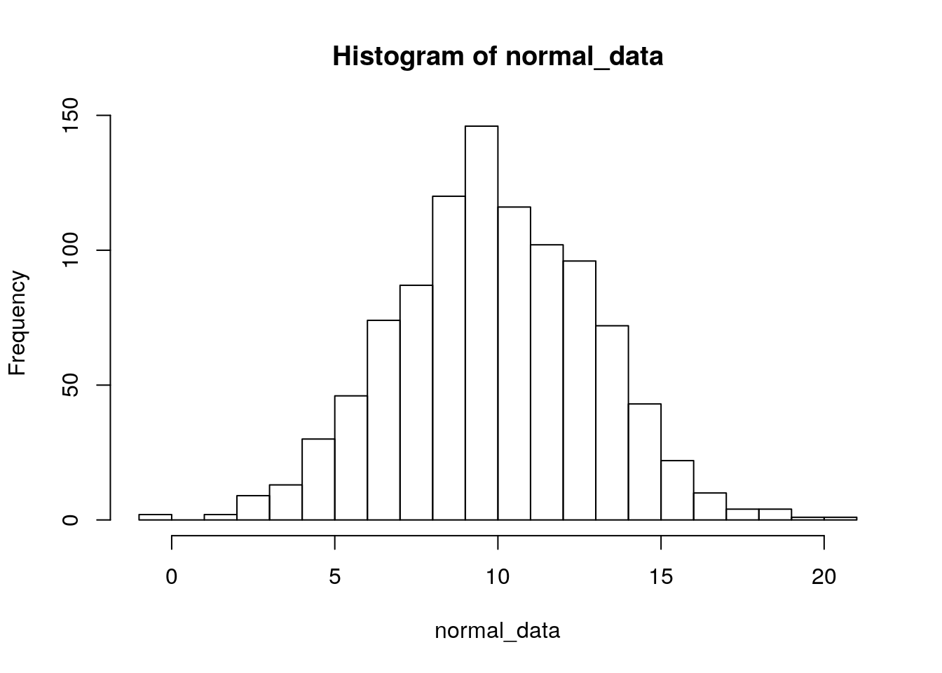
skewed_data <- rSHASHo2(n=1000,mu=10,sigma=3,nu=0.5,tau = 1)
hist(skewed_data,breaks=20)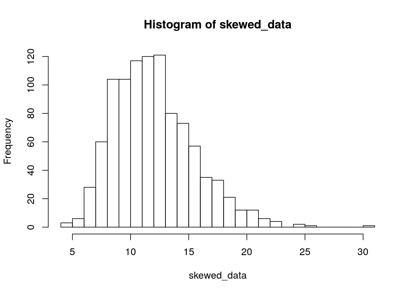
skewed_data <- rSHASHo(n=1000,mu=10,sigma=3,nu=-1,tau = 1)
hist(skewed_data,breaks=20)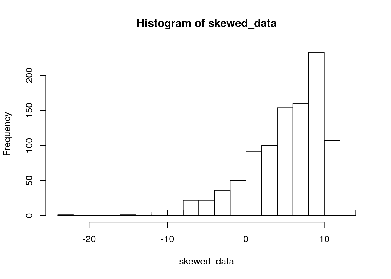
heavy_tailed_data <- rSHASHo(n=1000,mu=10,sigma=3,nu=0,tau = 0.5)
hist(heavy_tailed_data,breaks=20)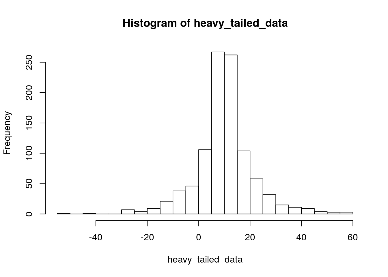
light_tailed_data <- rSHASHo(n=1000,mu=10,sigma=3,nu=0,tau = 1.5)
hist(light_tailed_data,breaks=20)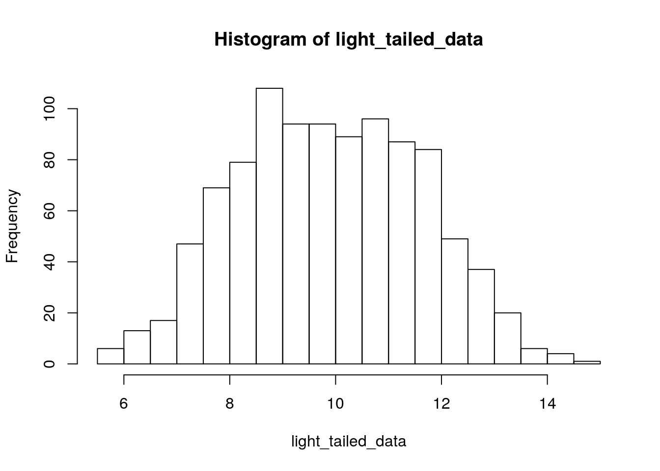 Now we can try out the same kinds of simulations as before:
reps <- 1e4
pvals <- rep(0,reps)
N <- 10
for (i in 1:reps) {
group1 <- rSHASHo(n=N,mu=10,sigma=3,nu=0,tau = 0.5)
group2 <- rSHASHo(n=N,mu=10,sigma=3,nu=0,tau = 1)
pvals[i] <- t.test(group1,group2,var.equal=TRUE)$p.value
}
sum(pvals<0.05)/reps
## [1] 0.0519reps <- 1e4
pvals <- rep(0,reps)
N1 <- 10
N2 <- 20
for (i in 1:reps) {
group1 <- rSHASHo(n=N1,mu=10,sigma=3,nu=0,tau = 0.5)
group2 <- rSHASHo(n=N2,mu=10,sigma=3,nu=0,tau = 1)
pvals[i] <- t.test(group1,group2,var.equal=TRUE)$p.value
}
sum(pvals<0.05)/reps## [1] 0.15077.3.3 Extreme non-normality: the Cauchy distribution
The Cauchy distribution can be used to simulate data from a distribution that takes on extreme outliers. The Cauchy distribution has no population mean or variance; the Law of Large Numbers and Central Limit Theorem do not “work” with the Cauchy distribution insofar as the sample mean never converges to a population mean, regardless of sample size. Here’s an example of data from a Cauchy distribution:
set.seed(335)
cauchy_data <- rcauchy(n=200,location=0,scale=1)
hist(cauchy_data,breaks=20)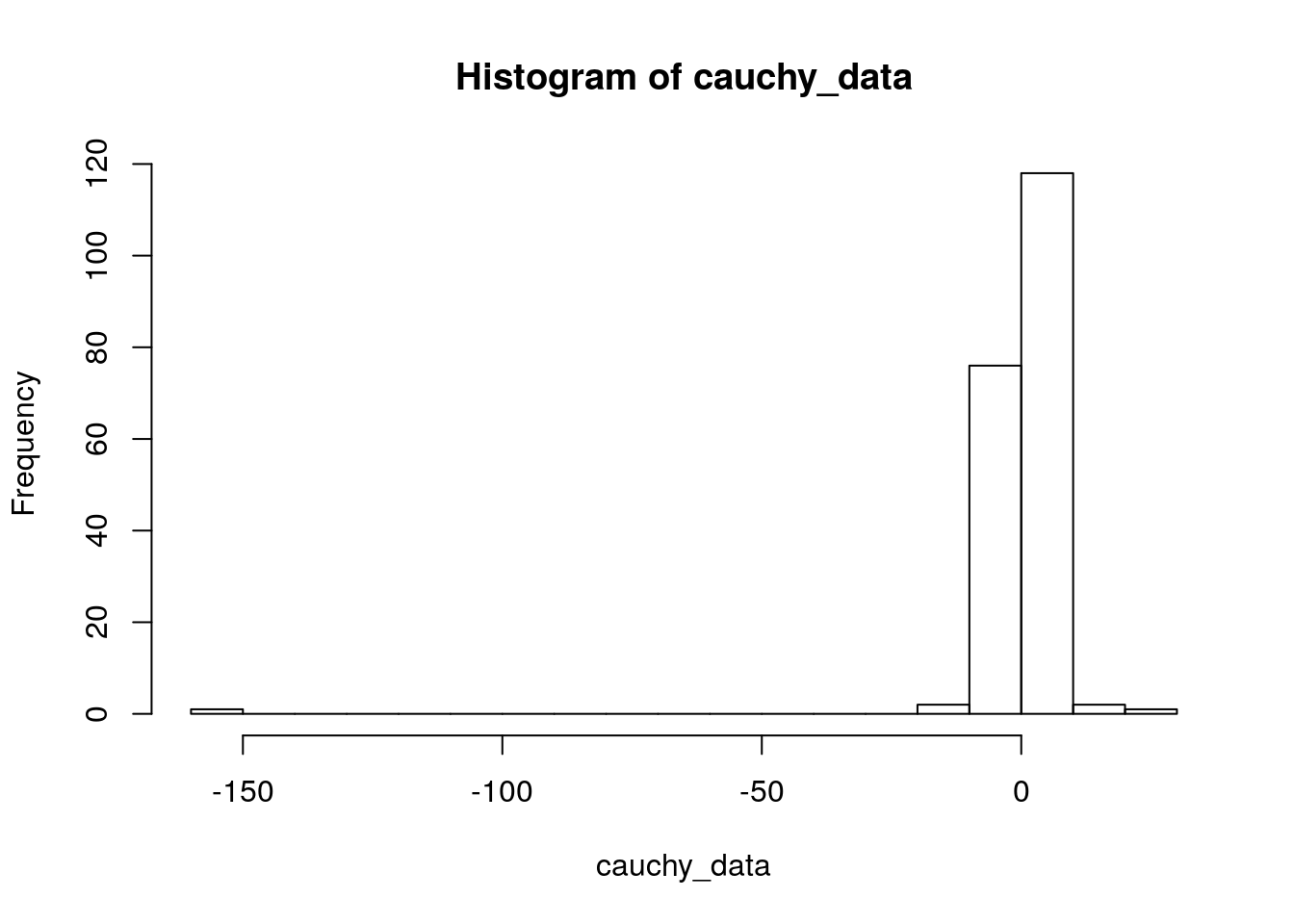
And again:
cauchy_data <- rcauchy(n=200,location=0,scale=1)
hist(cauchy_data,breaks=20)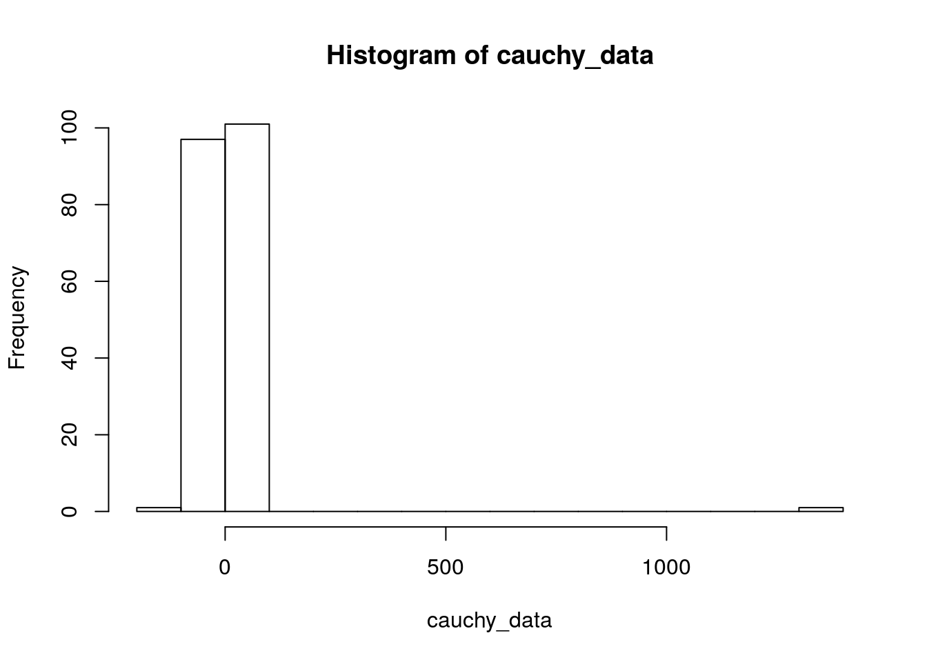
A Cauchy random variable can also be constructed as the ratio of two standard normal random variables:
normal_numerators <- rnorm(200)
normal_denominators <- rnorm(200)
Cauchy_from_normals <- normal_numerators/normal_denominators
hist(Cauchy_from_normals,breaks=20)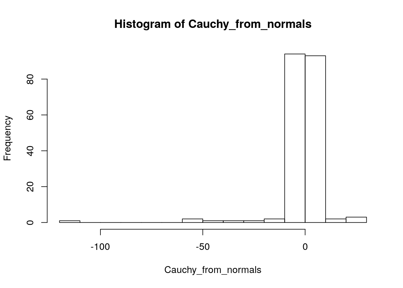
The Cauchy distribution’s “location” parameter is its median. Since the median isn’t sensitive to outliers, this parameter can be defined and is quite stable; the sample median is an unbiased estimator of the population median.
The Cauchy distribution’s “scale” parameter is its inter-quartile range. The IQR encloses the central 50% of values in a data set.
Let’s re-do our simulations, this time using the Cauchy distribution to model extreme non-normality:
reps <- 1e4
pvals <- rep(0,reps)
tstats <- rep(0,reps)
N <- 10
for (i in 1:reps) {
group1 <- rcauchy(n=N,location=0,scale=1)
group2 <- rcauchy(n=N,location=0,scale=1)
test_results <- t.test(group1,group2,var.equal=TRUE)
pvals[i] <- test_results$p.value
tstats[i] <- test_results$statistic
}
sum(pvals<0.05)/reps
## [1] 0.0213This is conservative. Changing the sample size won’t do anything. For fun, let’s look at the distribution of test statistics from this simulation:
hist(tstats)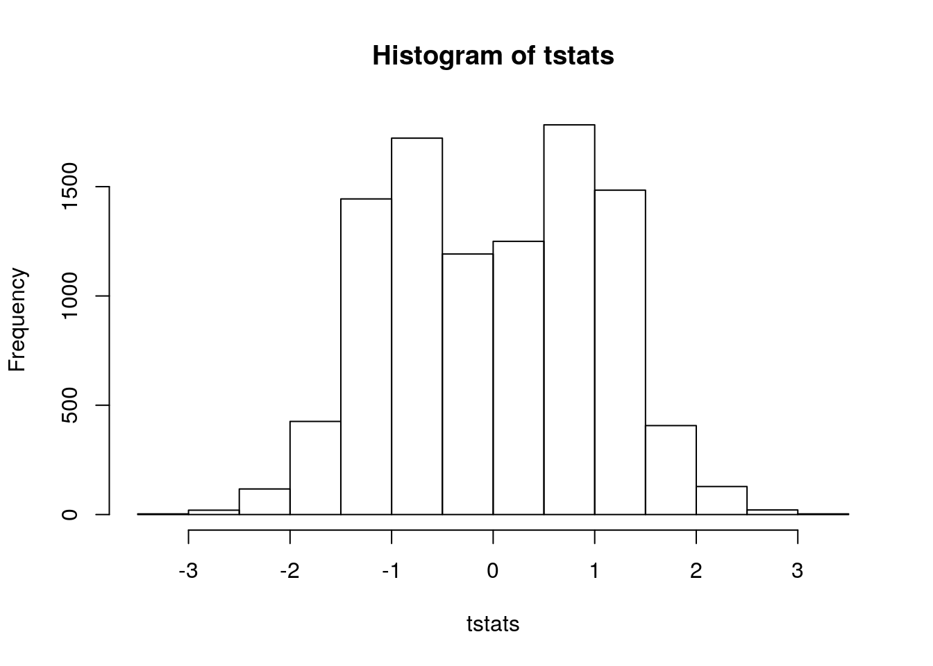
The Cauchy distribution is “heavy-tailed”: it produces outliers in both directions. There is also a “half-Cauchy” distribution that produces only positive values, and a “skewed Cauchy” with an adjustable skew parameter. But we’ll stop here.
7.3.4 Don’t “test” assumptions!
We’ve seen a few examples of model assumptions being broken in was that aren’t consequential for the purpose of drawing inference on parameters (note: they’d be consequential if we were just making predictions!). It is for this reason that it is not a good idea to conduct formal tests to check assumptions. For example:
Levene’s Test tests against the null hypothesis that population variance is the same for all values of our predictor variable. It can be found in the package lawstat, function levene.Test().
The Shapiro-Wilk test tests against the null hypothesis that a set of data came from a normal distribution. The function shapiro.test implements this.
Exercise: Go back to previous examples in this section and include these tests in the simulations. See if there are cases in which the tests report “significant” violations of model assumptions that are, nonetheless, inconsequential. We’ll do this for Shapiro-Wilk test here.
First, we’ll try it on normal data:
set.seed(335)
test_shapiro <- rnorm(n=100,mean=0,sd=1)
shapiro.test(test_shapiro)
##
## Shapiro-Wilk normality test
##
## data: test_shapiro
## W = 0.98606, p-value = 0.3773Now we’ll check that its Type I error rate is correct:
N <- 100
reps <- 1e4
shapiro_pvals <- rep(0,reps)
for (i in 1:reps) {
  test_shapiro <- rnorm(n=N,mean=0,sd=1)
  shapiro_pvals[i] <- shapiro.test(test_shapiro)$p.value
}

sum(shapiro_pvals<0.05)/reps
## [1] 0.0472Now let’s try it out on some non-normal data:
N <- 100
reps <- 1e4
shapiro_pvals <- rep(0,reps)
for (i in 1:reps) {
  test_shapiro <- rSHASHo(n=N,mu=10,sigma=3,nu=0,tau = 0.5)
  shapiro_pvals[i] <- shapiro.test(test_shapiro)$p.value
}

sum(shapiro_pvals<0.05)/reps
## [1] 0.9714That’s some high power! Let’s use it now on the residuals from one of our previous t-test simulations:
reps <- 1e4
pvals <- rep(0,reps)
shapiro_pvals <- rep(0,reps)
N <- 10
for (i in 1:reps) {
group1 <- rSHASHo(n=N,mu=10,sigma=3,nu=0,tau = 0.5)
group2 <- rSHASHo(n=N,mu=10,sigma=3,nu=0,tau = 1)
test_results <- t.test(group1,group2,var.equal=TRUE)
pvals[i] <- test_results$p.value
resids <- c(group1-mean(group1),group2-mean(group2))
shapiro_pvals[i] <- shapiro.test(resids)$p.value
}
sum(pvals<0.05)/reps
## [1] 0.05sum(shapiro_pvals<0.05)/reps## [1] 0.561In this case, the Shapiro-Wilk test has about 57% power to reject the null of normality. Also, in this case, violating the assumption of normality didn’t do anything bad to our Type I error rate.
7.4 Some practical examples
7.4.1 “The Birthday Problem”
This is a classic probability problem: how large a random sample of people do you need in order for there to be a better than 50% chance two will have the same birthday? The answer is surprisingly small; only 23. If you have 23 people, the probability that at least two will have the same birthday is 0.507, or 50.7%. The Wikipedia page explains the math and the intuition behind the answer, if you’re curious.
There is a false assumption made for the mathematical solution given on the Wikipedia page: we assume that all birthdays are equally likely. In other words, the probability distribution for the variable “what is this person’s birthday?” is uniform across the integers 1 through 365 (this problem also leaves out February 29th).
This is empirically false. There are fewer births on major holidays, and fewer births on weekends. There are also more fall births than spring births. Here is a detailed plot, taken from the cover of Gelman et. al’s textbook “Bayesian Data Analysis”:
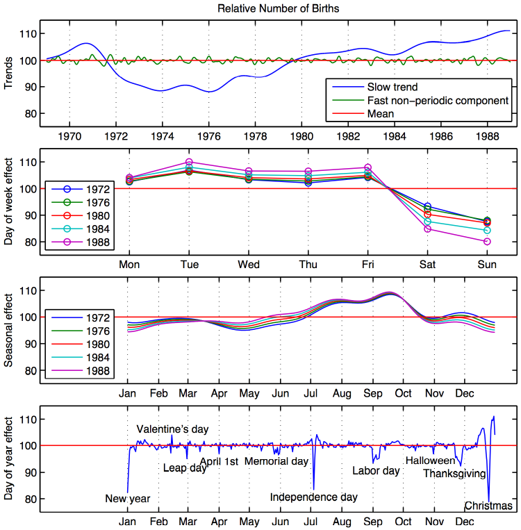
Since days of the year fall on different days of the week across years, this would only matter if we sampled people the same age. But, what about the fact that, in the USA, there are more fall births than spring births, and substantial declines on major holidays? What effect does violating our mathematical assumption have on the calculated result?
It turns out that the assumption of uniform probability is a “conservative” assumption in that it makes the number of people needed be as large as possible, or equivalently makes the calculated probability be as small as possible. So the true probability of having two or more people out of 23 with the same birthday is actually bigger than 50.7%.
It also turns out that, for this problem, the solution is still 23. The probability of at least two people out of 22 having the same birthday, assuming uniform probability, is 0.476 or 47.6%. And the empirical distribution of birthday probabilities does not differ from uniform by enough to push this value above 50%.
Here are a couple of articles explaining the adjustment for a non-uniform distribution of birthdays:
7.4.2 “No two decks of cards have ever been shuffled the same”
Link to one of many websites presenting this claim
Here is another (similar) probability question: what are the chances that two fair shuffles of a deck of 52 cards will produce the exact same ordering of cards? The answer is:
\[ \begin{split} \frac{1}{\text{The number of different ways to order a set of 52 cards}}& =\\ \frac{1}{52\cdot 51\cdot 50\cdot\ 49\cdot\ 48\cdot\ ...\ \cdot 6\cdot 5 \cdot 4\cdot 3\cdot 2\cdot 1} &=\\ \\ \frac{1}{52!}&=8\cdot 10^{-67} \end{split} \]
That’s a very small number, and human beings haven’t been shuffling cards for even a teeny tiny fraction of the time that would be needed in order to have a reasonable shot at two shuffles being exactly the same.
But, look at what is assumed here. We are assuming that the first card is a random draw from all 52 possible cards. And then, the second card is a random draw from the remaining 51 possible cards. And so on, until we get down to the final card.
Obviously this is not how human being shuffle cards. But, remember the theme of this chapter: just because a model assumption is false, doesn’t mean it is consequentially false. We just saw, for instance, that the false assumption underlying the solution to the birthday problem did not invalidate this solution. So, does it matter that the “pick one card completely at random from the remaining cards over and over again” model for card shuffling is false?
The answer this time is almost certainly “yes”. There is a lot of research on shuffling methods
Consider that most people don’t shuffle a deck well enough to approximate “true randomness”. According to some mathematicians who have studied this, 5 to 7 riffle shuffles are needed to achieve this (see, e.g. this article). Then consider that brand new decks of cards come in a set order. And that some games (e.g. bridge) involve placing like cards together before the next round is played. Now we have the combination of:
- Far from perfect shuffling methods
- Identical or similar starting orders from which imperfect shuffling methods are applied
Does this prove that there have, in fact, been at least two decks of cards throughout all of history that were shuffled into the same order? No, but it at least makes that \(8\cdot 10^{-67}\) figure irrelevant to the real-world version of the question.
7.4.3 Election polling
The paper “Disentangling bias and variance in election polling” compares stated margins of error from election polls with observed errors calculated from subsequent election results:
Here is an outline of the paper:
Statistical margins of error quantify estimation error expected from “random chance”. Consider a 95% margin of error. Conditional on some model assumptions, we can say that if we were to take new random samples from the same population over and over again, in 95% of samples the difference between the true population parameter value and its estimate will be less than the 95% margin of error.
There is more to error than statistical error. For example, our sampling method might make it more likely that certain subsets of the population are sampled than others. Or, certain subsets of the population may be more inclined to talk to pollsters than others. Or there may be data quality issues, e.g. some respondents lie or tell the pollster what they think the pollster wants to hear. Or, the state of public opinion on the day of the poll might change by the time the election takes place. These are all sources of error we’d call bias.
Response rates to polls are very low, less than 10%. So, small changes in non-statistical error could have a large impact on polls (e.g. the “convention boost”, almost certainly caused by supporters of the party who is currently having its convention being more motivated to respond to pollsters).
Non-statistical error (i.e. bias) is a concern in most applications, not just in polling. We usually have no way of measuring bias, because we never get to know the true parameter value we are estimating. Election polling is an interesting exception: we do get to find out the outcome of the election and the actual margin of victory for the winner.
So, the authors of this paper looked at a large number of historical polls taken shortly before an election, and compared the poll estimates to the observed election outcomes. The differences between poll estimates and actual outcomes are observed “errors”. The authors obtained a distribution of observed errors across many elections, and calculated the values that enclosed the central 95% of these errors.
The authors found that the observed 95% margins of error were about twice as large as the statistical margins of error. And so, amount of polling error due to “random chance” was comparable to the amount of polling error due to “bias”. Their advice: when you read the results of an election poll, take the stated margin of error and double it!
The authors also found very little systematic bias in polls toward one party or the other, though this may have changed in recent years.