4 Efficient workflow

Efficient programming is an important skill for generating the correct result, on time. Yet coding is only one part of a wider skillset needed for successful outcomes for projects involving R programming. Unless your project is to write generic R code (i.e. unless you are on the R Core Team), the project will probably transcend the confines of the R world: it must engage with a whole range of other factors. In this context we define ‘workflow’ as the sum of practices, habits and systems that enable productivity.⁹ To some extent workflow is about personal preferences. Everyone’s mind works differently so the most appropriate workflow varies from person to person and from one project to the next. Project management practices will also vary depending the scale and type of the project: it’s a big topic but can usefully be condensed in 5 top tips.

Prerequisites

This chapter focuses on workflow. For project planning and management, we’ll use the DiagrammeR package. For project reporting we’ll focus on R Markdown and knitr which are bundled with RStudio (but can be installed independently if needed). We’ll suggest other packages that are worth investigating, but are not required for this particular chapter.

library("DiagrammeR")

4.1 Top 5 tips for efficient workflow

Start without writing code but with a clear mind and perhaps a pen and paper. This will ensure you keep your objectives at the forefront of your mind, without getting lost in the technology.
Make a plan. The size and nature will depend on the project but time-lines, resources and ‘chunking’ the work will make you more effective when you start.
Select the packages you will use for implementing the plan early. Minutes spent researching and selecting from the available options could save hours in the future.
Document your work at every stage: work can only be effective if it’s communicated clearly and code can only be efficiently understood if it’s commented.
Make your entire workflow as reproducible as possible. knitr can help with this in the phase of documentation.

4.2 A project planning typology

Appropriate project management structures and workflow depend on the type of project you are undertaking. The typology below demonstrates the links between project type and project management requirements.¹⁰

Data analysis. Here you are trying to explore datasets to discover something interesting/answer some questions. The emphasis is on speed of manipulating your data to generate interest results. Formality is less important in this type of project. Sometimes this analysis project may only be part of a larger project (the data may have to be created in a lab, for example). How the data analysts interact with the rest of the team may be as important for the project’s success as how they interact with each other.
Package creation. Here you want to create code that can be reused across projects, possibly by people whose use case you don’t know (if you make it publicly available). The emphasis in this case will be on clarity of user interface and documentation, meaning style and code review are important. Robustness and testing are important in this type of project too.
Reporting and publishing. Here you are writing a report or journal paper or book. The level of formality varies depending upon the audience, but you have additional worries like how much code it takes to arrive at the conclusions, and how much output does the code create.
Software applications. This could range from a simple Shiny app to R being embedded in the server of a much larger piece of software. Either way, since there is limited opportunity for human interaction, the emphasis is on robust code and gracefully dealing with failure.

Based on these observations we recommend thinking about which type of workflow, file structure and project management system suits your projects best. Sometimes it’s best not to be prescriptive so we recommend trying different working practices to discover which works best, time permitting.¹¹

There are, however, concrete steps that can be taken to improve workflow in most projects that involve R programming. Learning them will, in the long-run, improve productivity and reproducibility. With these motivations in mind, the purpose of this chapter is simple: to highlight some key ingredients of an efficient R workflow. It builds on the concept of an R/RStudio project, introduced in Chapter 2, and is ordered chronologically throughout the stages involved in a typical project’s lifespan, from its inception to publication:

Project planning. This should happen before any code has been written, to avoid time wasted using a mistaken analysis strategy. Project management is the art of making project plans happen.
Package selection. After planning your project you should identify which packages are most suitable to get the work done quickly and effectively. With rapid increases in the number and performance of packages it is more important than ever to consider the range of options at the outset. For example *_join() from dplyr is often more appropriate than merge(), as we’ll see in 6.
Publication. This final stage is relevant if you want your R code to be useful for others in the long term. To this end Section 4.5 touches on documentation using knitr and the much stricter approach to code publication of package development.

4.3 Project planning and management

Good programmers working on a complex project will rarely just start typing code. Instead, they will plan the steps needed to complete the task as efficiently as possible: “smart preparation minimizes work” (Berkun 2005). Although search engines are useful for identifying the appropriate strategy, trail-and-error approaches (for example typing code at random and Googling the inevitable error messages) are usually highly inefficient.

Strategic thinking especially important during a project’s inception: if you make a bad decision early on, it will have cascading negative impacts throughout the project’s entire lifespan. So detrimental and ubiquitous is this phenomenon in software development that a term has been coined to describe it: technical debt. This has been defined as “not quite right code which we postpone making it right” (Kruchten, Nord, and Ozkaya 2012). Dozens of academic papers have been written on the subject but, from the perspective of beginning a project (i.e. in the planning stage, where we are now), all you need to know is that it is absolutely vital to make sensible decisions at the outset. If you do not, your project may be doomed to failure of incessant rounds of refactoring.

To minimise technical debt at the outset, the best place to start may be with a pen and paper and an open mind. Sketching out your ideas and deciding precisely what you want to do, free from the constraints of a particular piece of technology, can be rewarding exercise before you begin. Project planning and ‘visioning’ can be a creative process not always well-suited to the linear logic of computing, despite recent advances in project management software, some of which are outlined in the bullet points below.

Scale can loosely be defined as the number of people working on a project. It should be considered at the outset because the importance of project management increases exponentially with the number of people involved. Project management may be trivial for a small project but if you expect it to grow, implementing a structured workflow early could avoid problems later. On small projects consisting of a ‘one off’ script, project management may be a distracting waste of time. Large projects involving dozens of people, on the other hand, require much effort dedicated to project management: regular meetings, division of labour and a scalable project management system to track progress, issues and priorities will inevitably consume a large proportion of the project’s time. Fortunately a multitude of dedicated project management systems have been developed to cater for projects across a range of scales. These include, in rough ascending order of scale and complexity:

the interactive code sharing site GitHub, which is described in more detail in Chapter 9
ZenHub, a browser plugin that is “the first and only project management suite that works natively within GitHub”
web-based and easy-to-use tools such as Trello
dedicated desktop project management software such as ProjectLibre and GanttProject
fully featured, enterprise scale open source project management systems such as OpenProject and redmine.

Regardless of the software (or lack thereof) used for project management, it involves considering the project’s aims in the context of available resources (e.g. computational and programmer resources), project scope, time-scales and suitable software. And these things should be considered together. To take one example, is it worth the investment of time needed to learn a particular R package which is not essential to completing the project but which will make the code run faster? Does it make more sense to hire another programmer or invest in more computational resources to complete an urgent deadline?

Minutes spent thinking through such issues before writing a single line can save hours in the future. This is emphasised in books such as Berkun (2005) and PMBoK (2000) and useful online resources such those by teamgantt.com and lasa.org.uk, which focus exclusively on project planning. This section condenses some of the most important lessons from this literature in the context of typical R projects (i.e. which involve data analysis, modelling and visualisation).

4.3.1 ‘Chunking’ your work

Once a project overview has been devised and stored, in mind (for small projects, if you trust that as storage medium!) or written, a plan with a time-line can be drawn-up. The up-to-date visualisation of this plan can be a powerful reminder to yourself and collaborators of progress on the project so far. More importantly the timeline provides an overview of what needs to be done next. Setting start dates and deadlines for each task will help prioritise the work and ensure you are on track. Breaking a large project into smaller chunks is highly recommended, making huge, complex tasks more achievable and modular PMBoK (2000). ‘Chunking’ the work will also make collaboration easier, as we shall see in Chapter 5.

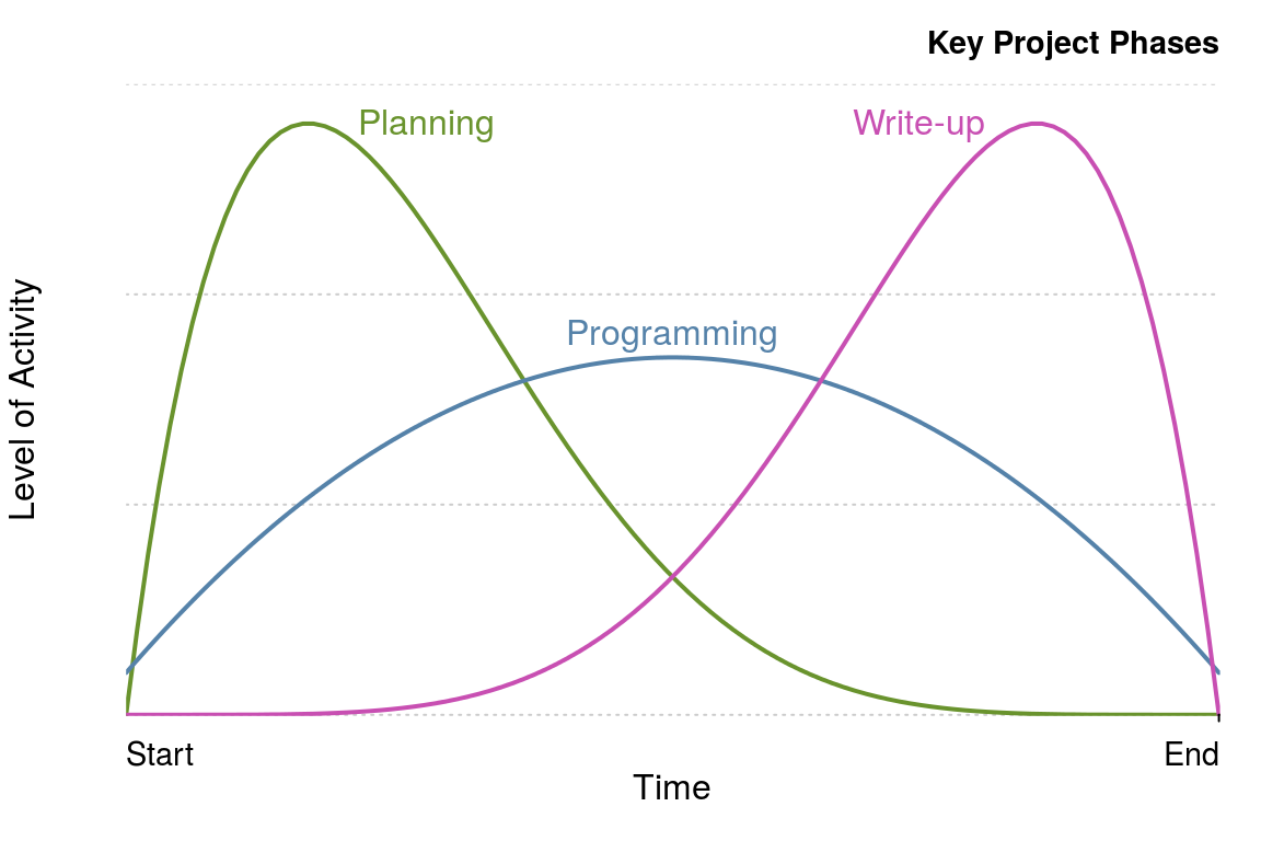
Figure 4.1: Schematic illustrations of key project phases and levels of activity over time, based on PMBoK (2000).

The tasks that a project should be split into will depend the nature of the work and the phases illustrated in Figure 4.1 represent a rough starting point, not a template and the ‘programming’ phase will usually need to be split into at least ‘data tidying’, ‘processing’, and ‘visualisation’.

4.3.2 Making your workflow SMART

A more rigorous (but potentially onerous) way to project plan is to divide the work into a series of objectives and tracking their progress throughout the project’s duration. One way to check if an objective is appropriate for action and review is by using the SMART criteria.

Specific: is the objective clearly defined and self-contained?
Measurable: is there a clear indication of its completion?
Attainable: can the target be achieved? This can also refer to Assigned (to a person).
Realistic: have sufficient resources been allocated to the task?
Time-bound: is there an associated completion date or milestone?

If the answer to each of these questions is ‘yes’, the task is likely to be suitable to include in the project’s plan. Note that this does not mean all project plans need to be uniform. A project plan can take many forms, including a short document, a Gantt chart (see Figure 4.2 or simply a clear vision of the project’s steps in mind.

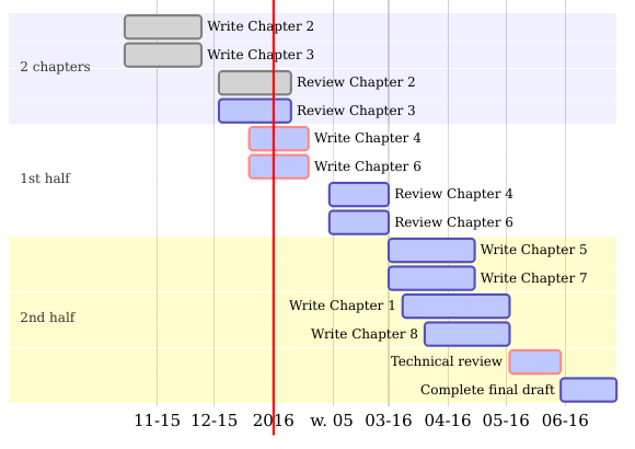
Figure 4.2: A Gantt chart created using DiagrammeR illustrating the steps needed to complete this book at an early stage of its development.

4.3.3 Visualising plans with R

Various R packages can help visualise the project plan. While these are useful, they cannot compete with the dedicated project management software outlined at the outset of this section. However, if you are working on relatively simple project, it is useful to know that R can help represent and keep track of your work. Packages for plotting project progress include:¹²

the plan package, which provides basic tools to create burndown charts (which concisely show whether a project is on-time or not) and Gantt charts.
plotrix, a general purpose plotting package, provides basic Gantt chart plotting functionality. Enter example(gantt.chart) for details.
DiagrammeR, a new package for creating network graphs and other schematic diagrams in R. This package provides an R interface to simple flow-chart file formats such as mermaid and GraphViz.

The small example below (which provides the basis for creating charts like Figure 4.2 illustrates how DiagrammeR can take simple text inputs to create informative up-to-date Gantt charts. Such charts can greatly help with the planning and task management of long and complex R projects, as long as they do not take away valuable programming time from core project objectives.

library("DiagrammeR")
# Define the Gantt chart and plot the result (not shown)
mermaid("gantt
        Section Initiation
        Planning           :a1, 2016-01-01, 10d
        Data processing    :after a1  , 30d")

In the above code gantt defines the subsequent data layout. Section refers to the project’s section (useful for large projects, with milestones) and each new line refers to a discrete task. Planning, for example, has the code a, begins on the first day of 2016 and lasts for 10 days. See knsv.github.io/mermaid/gantt.html for more detailed documentation.

Exercises

What are the three most important work ‘chunks’ of your current R project?
What is the meaning of ‘SMART’ objectives (see Making your workflow SMART).
Run the code chunk at the end of this section to see the output.
Bonus exercise: modify this code to create a basic Gantt chart of an R project you are working on.

4.4 Package selection

A good example of the importance of prior planning to minimise effort and reduce technical debt is package selection. An inefficient, poorly supported or simply outdated package can waste hours. When a more appropriate alternative is available this waste can be prevented by prior planning. There are many poor packages on CRAN and much duplication so it’s easy to go wrong. Just because a certain package can solve a particular problem, doesn’t mean that it should.

Used well, however, packages can greatly improve productivity: not reinventing the wheel is part of the ethos of open source software. If someone has already solved a particular technical problem, you don’t have to re-write their code, allowing you to focus on solving the applied problem. Furthermore, because R packages are generally (but not always) written by competent programmers and subject to user feedback, they may work faster and more effectively that the hastily prepared code you may have written. All R code is open source and potentially subject to peer review. A prerequisite of publishing an R package is that developer contact details must be provided, and many packages provide a site for issue tracking. Furthermore, R packages can increase programmer productivity by dramatically reducing the amount of code they need to write because all the code is packaged in functions behind the scenes.

Let’s take an example. Imagine for a project you would like to find the distance between sets of points (origins, o and destinations, d) on the Earth’s surface. Background reading shows that a good approximation of ‘great circle’ distance, which accounts for the curvature of the Earth, can be made by using the Haversine formula, which you duly implement, involving much trial and error:

# Function to convert degrees to radians
deg2rad = function(deg) deg * pi / 180

# Create origins and destinations
o = c(lon = -1.55, lat = 53.80)
d = c(lon = -1.61, lat = 54.98)

# Convert to radians
o_rad = deg2rad(o)
d_rad = deg2rad(d)

# Find difference in degrees
delta_lon = (o_rad[1] - d_rad[1])
delta_lat = (o_rad[2] - d_rad[2])

# Calculate distance with Haversine formula
a = sin(delta_lat / 2)^2 + cos(o_rad[2]) * cos(d_rad[2]) * sin(delta_lon / 2)^2
c = 2 * asin(min(1, sqrt(a)))
(d_hav1 = 6371 * c) # multiply by Earth's diameter
#> [1] 131

This method works but it takes time to write, test and debug. Much better to package it up into a function. Or even better, use a function that someone else has written and put in a package:

# Find great circle distance with geosphere
(d_hav2 = geosphere::distHaversine(o, d))
#> [1] 131415

The difference between the hard-coded method and the package method is striking. One is 7 lines of tricky R code involving many subsetting stages and small, similar functions (e.g. sin and asin) which are easy to confuse. The other is one line of simple code. The package method using geosphere took perhaps 100^th of the time and gave a more accurate result (because it uses a more accurate estimate of the diameter of the Earth). This means that a couple of minutes searching for a package to estimate great circle distances would have been time well spent at the outset of this project. But how do you search for packages?

4.4.1 Searching for R packages

Building on the example above, how can on find out if there is a package to solve your particular problem? The first stage is to guess: if it is a common problem, someone has probably tried to solve it. The second stage is to search. A simple Google query, haversine formula R, returned a link to the geosphere package in the second result (a hardcoded implementation was first).

Beyond Google, there are also several sites for searching for packages and functions. rdocumentation.org provides a multi-field search environment to pinpoint the function or package you need. Amazingly, the search for haversine in the Description field yielded 10 results from 8 packages: R has at least 8 implementations of the Haversine formula! This shows the importance of careful package selection as there are often many packages that do the same job, as we see in the next section. There is also a way to find the function from within R, with RSiteSearch(), which opens a url in your browser linking to a number of functions (40) and vignettes (2) that mention the text string:

# Search CRAN for mentions of haversine
RSiteSearch("haversine")

4.4.2 How to select a package

Due to the conservative nature of base R development, which rightly prioritises stability over innovation, much of the innovation and performance gains in the ‘R ecosystem’ has occurred in recent years in the packages. The increased ease of package development (H. Wickham 2015 c) and interfacing with other languages (e.g. Eddelbuettel et al. 2011) has accelerated their number, quality and efficiency. An additional factor has been the growth in collaboration and peer review in package development, driven by code-sharing websites such as GitHub and online communities such as ROpenSci for peer reviewing code.

Performance, stability and ease of use should be high on the priority list when choosing which package to use. Another more subtle factor is that some packages work better together than others. The ‘R package ecosystem’ is composed of interrelated package. Knowing something of these inter-dependencies can help select a ‘package suite’ when the project demands a number of diverse yet interrelated programming tasks. The ‘tidyverse’, for example, contains many interrelated packages that work well together, such as readr, tidyr, and dplyr.¹³ These may be used together to read-in, tidy and then process the data, as outlined in the subsequent sections.

There is no ‘hard and fast’ rule about which package you should use and new packages are emerging all the time. The ultimate test will be empirical evidence: does it get the job done on your data? However, the following criteria should provide a good indication of whether a package is worth an investment of your precious time, or even installing on your computer:

Is it mature? The more time a package is available, the more time it will have for obvious bugs to be ironed out. The age of a package on CRAN can be seen from its Archive page on CRAN. We can see from cran.r-project.org/src/contrib/Archive/ggplot2/, for example, that ggplot2 was first released on the 10^th June 2007 and that it has had 29 releases. The most recent of these at the time of writing was ggplot2 2.1.0: reaching 1 or 2 in the first digit of package versions is usually an indication from the package author that the package has reached a high level of stability.
Is it actively developed? It is a good sign if packages are frequently updated. A frequently updated package will have its latest version ‘published’ recently on CRAN. The CRAN package page for ggplot2, for example, said Published: 2016-03-01, less than a six months old at the time of writing.
Is it well documented? This is not only an indication of how much thought, care and attention has gone into the package. It also has a direct impact on its ease of use. Using a poorly documented package can be inefficient due to the hours spent trying to work out how to use it! To check if the package is well documented, look at the help pages associated with its key functions (e.g. ?ggplot), try the examples (e.g. example(ggplot)) and search for package vignettes (e.g. vignette(package = "ggplot2")).
Is it well used? This can be seen by searching for the package name online. Most packages that have a strong user base will produce thousands of results when typed into a generic search engine such as Google’s. More specific (and potentially useful) indications of use will narrow down the search to particular users. A package widely used by the programming community will likely visible GitHub. At the time of writing a search for ggplot2 on GitHub yielded over 400 repositories and almost 200,000 matches in committed code! Likewise, a package that has been adopted for use in academia will tend to be mentioned in Google Scholar (again, ggplot2 scores extremely well in this measure, with over 5000 hits).

An article in simplystats discusses this issue with reference to the proliferation of GitHub packages (those that are not available on CRAN). In this context well-regarded and experienced package creators and ‘indirect data’ such as amount of GitHub activity are also highlighted as reasons to trust a package.

The websites of MRAN and METACRAN can help the package selection process by providing further information on each package uploaded to CRAN. METACRAN, for example, provides metadata about R packages via a simple API and the provision of ‘badges’ to show how many downloads a particular package has per month. Returning to the Haversine example above, we could find out how many times two packages that implement the formula are downloaded each month with the following urls:

http://cranlogs.r-pkg.org/badges/last-month/geosphere, downloads of geosphere:

http://cranlogs.r-pkg.org/badges/last-month/geoPlot, downloads of geoPlot:

It is clear from the results reported above that geosphere is by far the more popular package, so is a sensible and mature choice for dealing with distances on the Earth’s surface.

4.5 Publication

The final stage in a typical project workflow is publication. Although it’s the final stage to be worked on, that does not mean you should only document after the other stages are complete: making documentation integral to your overall workflow will make this stage much easier and more efficient.

Whether the final output is a report containing graphics produced by R, an online platform for exploring results or well-documented code that colleagues can use to improve their workflow, starting it early is a good plan. In every case the programming principles of reproducibility, modularity and DRY (don’t repeat yourself) will make your publications faster to write, easier to maintain and more useful to others.

Instead of attempting a comprehensive treatment of the topic we will touch briefly on a couple of ways of documenting your work in R: dynamic reports and R packages. There is a wealth of material on each of these online. A wealth of online resources exists on each of these; to avoid duplication of effort the focus is on documentation from a workflow efficiency perspective.

4.5.1 Dynamic documents with R Markdown

When writing a report using R outputs a typical workflow has historically been to 1) do the analysis 2) save the resulting graphics and record the main results outside the R project and 3) open a program unrelated to R such as LibreOffice to import and communicate the results in prose. This is inefficient: it makes updating and maintaining the outputs difficult (when the data changes, steps 1 to 3 will have to be done again) and there is an overhead involved in jumping between incompatible computing environments.

To overcome this inefficiency in the documentation of R outputs the R Markdown framework was developed. Used in conjunction with the knitr package, we have the ability to

process code chunks (via knitr)
a notebook interface for R (via RStudio)
the ability to render output to multiple formats (via pandoc).

R Markdown documents are plain text and have file extension .Rmd. This framework allows for documents to be generated automatically. Furthermore, nothing is efficient unless you can quickly redo it. Documenting your code inside dynamic documents in this way ensures that analysis can be quickly re-run.

This note briefly explains R Markdown for the un-initiated. R markdown is a form of Markdown. Markdown is a pure text document format that has become a standard for documentation for software. It is the default format for displaying text on GitHub. R Markdown allows the user to embed R code in a Markdown document. This is a powerful addition to Markdown, as it allows custom images, tables and even interactive visualisations, to be included in your R documents. R Markdown is an efficient file format to write in because it is light-weight, human and computer readable, and is much less verbose than HTML, LaTeX. This book was written in R Markdown.

In an R Markdown document, results are generated on the fly by including ‘code chunks’. Code chunks are R code that are preceded by ```{r, options} on the line before the R code, and ``` at the end of the chunk. For example, suppose we have the code chunk

```{r eval = TRUE, echo = TRUE}
(1:5)^2
```

in an R Markdown document. The eval = TRUE in the code indicates that the code should be evaluated while echo = TRUE controls whether the R code is displayed. When we compile the document, we get

(1:5)^2
#> [1]  1  4  9 16 25

R Markdown via knitr provides a wide range of options to customise what is displayed and evaluated. When you adapt to this workflow it is highly efficient, especially as RStudio provides a number of shortcuts that make it easy to create and modify code chunks. To create a chunk while editing a .Rmd file, for example, simply enter Ctrl/Cmd+Alt+I on Windows or Linux or select the option from the Code drop down menu.

Once your document has compiled it should appear on your screen into the file format requested. If a html file has been generated (as is the default), RStudio provides a feature that allows you to put it up online rapidly. This is done using the rpubs website, a store of a huge number of dynamic documents (which could be a good source of inspiration for your publications). Assuming you have an RStudio account, clicking the ‘Publish’ button at the top of the html output window will instantly publish your work online, with a minimum of effort, enabling fast and efficient communication with many collaborators and the public.

An important advantage of dynamically documenting work this way is that when the data or analysis code changes, the results will be updated in the document automatically. This can save hours of fiddly copying and pasting of R output between different programs. Also, if your client wants pages and pages of documented output, knitr can provide them with a minimum of typing, e.g. by creating slightly different versions of the same plot over and over again. From a delivery of content perspective, that is certainly an efficiency gain compared with hours of copying and pasting figures!

If your R Markdown documents include time-consuming processing stages, a speed boost can be attained after the first build by setting opts_chunk$set(cache = TRUE) in the first chunk of the document. This setting was used to reduce the build times of this book, as can be seen on GitHub.

Furthermore dynamic documents written in R Markdown can compile into a range of output formats including html, pdf and Microsoft’s docx. There is a wealth of information on the details of dynamic report writing that is not worth replicating here. Key references are RStudio’s excellent website on R Markdown hosted at rmarkdown.rstudio.com and, for a more detailed account of dynamic documents with R, (Xie 2015).

4.5.2 R packages

A strict approach to project management and workflow is treating your projects as R packages. This approach has advantages and limitations. The major risk with treating a project as a package is that the package is quite a strict way of organising work. Packages are suited for code intensive projects where code documentation is important. An intermediate approach is to use a ‘dummy package’ that includes a DESCRIPTION file in the root directory telling users of the project which packages must be installed for the code to work. This book is based on a dummy package so that we can easily keep the dependencies up-to-date (see the book’s DESCRIPTION file online for an insight into how this works).

Creating packages is good practice in terms of learning to correctly document your code, store example data, and even (via vignettes) ensure reproducibility. But it can take a lot of extra time so should not be taken lightly. This approach to R workflow is appropriate for managing complex projects which repeatedly use the same routines which can be converted into functions. Creating project packages can provide foundation for generalising your code for use by others, e.g. via publication on GitHub or CRAN. And R package development has been made much easier in recent years by the development of the devtools package, which is highly recommended for anyone attempting to write an R package.

The number of essential elements of R packages differentiate them from other R projects. Three of these are outlined below from an efficiency perspective.

The DESCRIPTION file contains key information about the package, including which packages are required for the code contained in your package to work, e.g. using Imports:. This is efficient because it means that anyone who installs your package will automatically install the other packages that it depends on.
The R/ folder contains all the R code that defines your package’s functions. Placing your code in a single place and encouraging you to make your code modular in this way can greatly reduce duplication of code on large projects. Furthermore the documentation of R packages through Roxygen tags such as #' This function does this... makes it easy for others to use your work. This form of efficient documentation is facilitated by the roxygen2 package.
The data/ folder contains example code for demonstrating to others how the functions work and transporting datasets that will be frequently used in your workflow. Data can be added automatically to your package project using the devtools package, with devtools::use_data(). This can increase efficiency by providing a way of distributing small to medium sized datasets and making them available when the package is loaded with the function data("data_set_name").

The package testthat makes it easier than ever to test your R code as you go, ensuring that nothing breaks. This, combined with ‘continuous integration’ services, such as that provided by Travis, make updating your code base as efficient and robust as possible. This, and more, is described in (Cotton 2016 b).

As with dynamic documents, package development is a large topic. For small ‘one-off’ projects the time taken in learning how to set-up a package may not be worth the savings. However packages provide a rigorous way of storing code, data and documentation that can greatly boost productivity in the long-run. For more on R packages see (H. Wickham 2015 c): the online version provides all you need to know about writing R packages for free (see r-pkgs.had.co.nz/).

References

Berkun, Scott. 2005. The Art of Project Management. O’Reilly Media.

Kruchten, Philippe, Robert L Nord, and Ipek Ozkaya. 2012. “Technical Debt: From Metaphor to Theory and Practice.” IEEE Software, no. 6. IEEE: 18–21.

PMBoK, A. 2000. “Guide to the Project Management Body of Knowledge.” Project Management Institute, Pennsylvania USA.

Wickham, Hadley. 2015c. R Packages. O’Reilly Media.

Eddelbuettel, Dirk, Romain François, J. Allaire, John Chambers, Douglas Bates, and Kevin Ushey. 2011. “Rcpp: Seamless R and C++ Integration.” Journal of Statistical Software 40 (8): 1–18.

Xie, Yihui. 2015. Dynamic Documents with R and Knitr. Vol. 29. CRC Press.

Cotton, Richard. 2016b. Testing R Code.

The Oxford Dictionary’s definition of workflow is similar, with a more industrial feel: “The sequence of industrial, administrative, or other processes through which a piece of work passes from initiation to completion.”↩
Thanks to Richard Cotton for suggesting this typology.↩
The importance of workflow has not gone unnoticed by the R community and there are a number of different suggestions to boost R productivity. Rob Hyndman, for example, advocates the strategy of using four self-contained scripts to break up R work into manageable chunks: load.R, clean.R, func.R and do.R.↩
For a more comprehensive discussion of Gantt charts in R, please refer to stackoverflow.com/questions/3550341.↩
An excellent overview of the ‘tidyverse’, formerly now as the ‘hadleyverse’ and its benefits is available from barryrowlingson.github.io/hadleyverse.↩