5 Efficient input/output

This chapter explains how to efficiently read and write data in R. Input/output (I/O) is the technical term for reading and writing data: the process of getting information into a particular computer system (in this case R) and then exporting it to the ‘outside world’ again (in this case as a file format that other software can read). Data I/O will be needed on projects where data comes from, or goes to, external sources. However, the majority of R resources and documentation start with the optimistic assumption that your data has already been loaded, ignoring the fact that importing datasets into R, and exporting them to the world outside the R ecosystem, can be a time-consuming and frustrating process. Tricky, slow or ultimately unsuccessful data I/O can cripple efficiency right at the outset of a project. Conversely, reading and writing your data efficiently will make your R projects more likely to succeed in the outside world.

The first section introduce rio, a ‘meta package’ for efficiently reading and writing data in a range of file formats. rio requires only two intuitive functions for data I/O, making it efficient to learn and use. Next we explore in more detail efficient functions for reading in files stored in common plain text file formats from the readr and data.table packages. Binary formats, which can dramatically reduce file sizes and read/write times, are covered next.

With the accelerating digital revolution and growth in open data, an increasing proportion of the world’s data can be downloaded from the internet. This trend is set to continue, making section 5.5, on downloading and importing data from the web, important for ‘future-proofing’ you I/O skills. The benchmarks in this chapter demonstrate that choice of file format and packages for data I/O can have a huge impact on computational efficiency.

Before reading in a single line of data, it is worth considering a general principle for reproducible data management: never modify raw data files. Raw data should be seen as read-only, and contain information about its provenance. Keeping the original file name and commenting on its origin are a couple of ways to improve reproducibility, even when the data are not publicly available.

Prerequisites

R can read data from a variety of sources. We begin by discussing the generic package rio that handles a wide variety of data types. Special attention is paid to CSV files, which leads to the readr and data.table packages. The relatively new package feather is introduced as binary file format, that has cross-language support.

library("rio")
library("readr")
library("data.table")
library("feather")

We also use the WDI package to illustrate accessing online data sets

library("WDI")

5.1 Top 5 tips for efficient data I/O

1. If possible, keep the names of local files downloaded from the internet or copied onto your computer unchanged. This will help you trace the provenance of the data in the future.

2. R’s native file format is .Rds. These files can be imported and exported using readRDS() and saveRDS() for fast and space efficient data storage.

3. Use import() from the rio package to efficiently import data from a wide range of formats, avoiding the hassle of loading format-specific libraries.

4. Use readr or data.table equivalents of read.table() to efficiently import large text files.

5. Use file.size() and object.size() to keep track of the size of files and R objects and take action if they get too big.

5.2 Versatile data import with rio

rio is a ‘A Swiss-Army Knife for Data I/O’. rio provides easy-to-use and computationally efficient functions for importing and exporting tabular data in a range of file formats. As stated in the package’s vignette, rio aims to “simplify the process of importing data into R and exporting data from R.” The vignette goes on to to explain how many of the functions for data I/O described in R’s Data Import/Export manual are out of date (for example referring to WriteXLS but not the more recent readxl package) and difficult to learn.

This is why rio is covered at the outset of this chapter: if you just want to get data into R, with a minimum of time learning new functions, there is a fair chance that rio can help, for many common file formats. At the time of writing, these include .csv, .feather, .json, .dta, .xls, .xlsx and Google Sheets (see the package’s github page for up-to-date information). Below we illustrate the key rio functions of import() and export():

library("rio")
# Specify a file
fname = system.file("extdata/voc_voyages.tsv", package = "efficient")
# Import the file (uses the fread function from data.table)
voyages = import(fname)
# Export the file as an Excel spreadsheet
export(voyages, "voc_voyages.xlsx")

There was no need to specify the optional format argument for data import and export functions because this is inferred by the suffix, in the above example .tsv and .xlsx respectively. You can override the inferred file format for both functions with the format argument. You could, for example, create a comma-delimited file called voc_voyages.xlsx with export(voyages, "voc_voyages.xlsx", format = "csv"). However, this would not be a good idea: it is important to ensure that a file’s suffix matches it’s format.

To provide another example, the code chunk below downloads and imports as a data frame information about the countries of the world stored in .json (downloading data from the internet is covered in more detail in Section 5.5):

capitals = import("https://github.com/mledoze/countries/raw/master/countries.json")

The ability to import and use .json data is becoming increasingly common as it a standard output format for many APIs. The jsonlite and geojsonio packages have been developed to make this as easy as possible.

Exercises

1. The final line in the code chunk above shows a neat feature of rio and some other packages: the output format is determined by the suffix of the file-name, which make for concise code. Try opening the voc_voyages.xlsx file with an editor such as LibreOffice Calc or Microsoft Excel to ensure that the export worked, before removing this rather inefficient file format from your system:

   file.remove("voc_voyages.xlsx")

2. Try saving the the voyages data frames into 3 other file formats of your choosing (see vignette("rio") for supported formats). Try opening these in external programs. Which file formats are more portable?

3. As a bonus exercise, create a simple benchmark to compare the write times for the different file formats used to complete the previous exercise. Which is fastest? Which is the most space efficient?

5.3 Plain text formats

‘Plain text’ data files are encoded in a format (typically UTF-8) that can be read by humans and computers alike. The great thing about plain text is their simplicity and their ease of use: any programming language can read a plain text file. The most common plain text format is .csv, comma-separated values, in which columns are separated by commas and rows are separated by line breaks. This is illustrated in the simple example below:

Person, Nationality, Country of Birth
Robin, British, England
Colin, British, Scotland

There is often more than one way to read data into R and .csv files are no exception. The method you choose has implications for computational efficiency. This section investigates methods for getting plain text files into R, with a focus on three approaches: base R’s plain text reading functions such as read.csv(); the data.table approach, which uses the function fread(); and the newer readr package which provides read_csv() and other read_*() functions such as read_tsv(). Although these functions perform differently, they are largely cross-compatible, as illustrated in the below chunk, which loads data on the concentration of CO² in the atmosphere over time:

In general, you should never “hand-write” a CSV file. Instead, you should use write.csv() or an equivalent function. The Internet Engineering Task Force has the CSV definition that facilities sharing CSV files between tools and operating systems.

df_co2 = read.csv("extdata/co2.csv")
df_co2_dt = readr::read_csv("extdata/co2.csv")
#> Warning: Missing column names filled in: 'X1' [1]
#> Parsed with column specification:
#> cols(
#>   X1 = col_integer(),
#>   time = col_double(),
#>   co2 = col_double()
#> )
df_co2_readr = data.table::fread("extdata/co2.csv")

Note that a function ‘derived from’ another in this context means that it calls another function. The functions such as read.csv() and read.delim() in fact are wrappers around read.table(). This can be seen in the source code of read.csv(), for example, which shows that the function is roughly the equivalent of read.table(file, header = TRUE, sep = “,”).

Although this section is focussed on reading text files, it demonstrate the wider principle that the speed and flexibility advantages of additional read functions can be offset by the disadvantages of addition package dependency (in terms of complexity and maintaining the code) for small datasets. The real benefits kick in on large datasets. Of course, there are some data types that require a certain package to load in R: the readstata13 package, for example, was developed solely to read in .dta files generated by versions of Stata 13 and above.

Figure 5.1 demonstrates that the relative performance gains of the data.table and readr approaches increase with data size, especially so for data with many rows. Below around \(1\) MB read.csv() is actually faster than read_csv() while fread is much faster than both, although these savings are likely to be inconsequential for such small datasets.

For files beyond \(100\) MB in size fread() and read_csv() can be expected to be around 5 times faster than read.csv(). This efficiency gain may be inconsequential for a one-off file of \(100\) MB running on a fast computer (which still takes less than a minute with read.csv()), but could represent an important speed-up if you frequently load large text files.

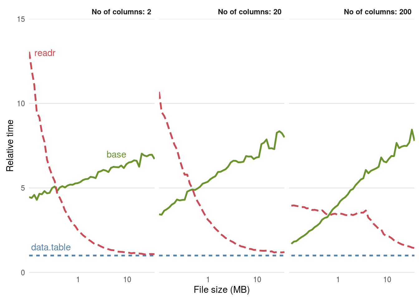
Figure 5.1: Benchmarks of base, data.table and readr approches for reading csv files, using the functions read.csv(), fread() and read_csv(), respectively. The facets ranging from \(2\) to \(200\) represent the number of columns in the csv file.

When tested on a large (\(4\)GB) .csv file it was found that fread() and read_csv() were almost identical in load times and that read.csv() took around \(5\) times longer. This consumed more than \(10\)GB of RAM, making it unsuitable to run on many computers (see Section 8.3 for more on memory). Note that both readr and base methods can be made significantly faster by pre-specifying the column types at the outset (see below). Further details are provided by the help in ?read.table.

read.csv(file_name, colClasses = c("numeric", "numeric"))

In some cases with R programming there is a trade-off between speed and robustness. This is illustrated below with reference to differences in how readr, data.table and base R approaches handle unexpected values. Figure 5.1 highlights that as the dataset size increases, the benefit of switching to fread() and (eventually) to read_csv() . For a small (\(1\)MB) dataset: fread() is around \(5\) times faster than base R.

5.3.1 Differences between fread() and read_csv()

The file voc_voyages was taken from a dataset on Dutch naval expeditions used with permission from the CWI Database Architectures Group. The data is described more fully at monetdb.org. From this dataset we primarily use the ‘voyages’ table with lists Dutch shipping expeditions by their date of departure.

fname = system.file("extdata/voc_voyages.tsv", package = "efficient")
voyages_base = read.delim(fname)

When we run the equivalent operation using readr,

voyages_readr = readr::read_tsv(fname)
#> Parsed with column specification:
#> cols(
#>   .default = col_character(),
#>   number = col_integer(),
#>   trip = col_integer(),
#>   tonnage = col_integer(),
#>   departure_date = col_date(format = ""),
#>   cape_arrival = col_date(format = ""),
#>   cape_departure = col_date(format = ""),
#>   arrival_date = col_date(format = ""),
#>   next_voyage = col_integer()
#> )
#> See spec(...) for full column specifications.
#> Warning: 2 parsing failures.
#>  row            col   expected  actual
#> 4403 cape_arrival   date like  2-01-01
#> 4592 cape_departure date like  8-05-17

a warning is raised regarding row 2841 in the built variable. This is because read_*() decides what class each variable is based on the first \(1000\) rows, rather than all rows, as base read.*() functions do. Printing the offending element

voyages_base$built[2841] # a factor.
#> [1] 1721-01-01
#> 182 Levels:  1135 1594 1600 1612 1613 1614 1615 1619 1620 1621 ... taken 1672
voyages_readr$built[2841] # an NA: text cannot be converted to numeric
#> [1] "1721-01-01"

Reading the file using data.table

# Verbose warnings not shown
voyages_dt = data.table::fread(fname)

generates 5 warning messages stating that columns 2, 4, 9, 10 and 11 were Bumped to type character on data row ..., with the offending rows printed in place of .... Instead of changing the offending values to NA, as readr does for the built column (9), fread() automatically converts any columns it thought of as numeric into characters. An additional feature of fread is that it can read-in a selection of the columns, either by their index or name, using the select argument. This is illustrated below by reading in only half (the first 11) columns from the voyages dataset and comparing the result with fread()’ing all the columns in.

microbenchmark(times = 5,
  with_select = data.table::fread(fname, select = 1:11),
  without_select = data.table::fread(fname)
)
#> Unit: milliseconds
#>            expr   min   lq  mean median   uq   max neval cld
#>     with_select  5.88  6.0  6.19   6.18  6.2  6.66     5  a 
#>  without_select 10.09 10.1 10.94  10.43 11.2 12.83     5   b

To summarise, the differences between base, readr and data.table functions for reading in data go beyond code execution times. The functions read_csv() and fread() boost speed partially at the expense of robustness because they decide column classes based on a small sample of available data. The similarities and differences between the approaches are summarised for the Dutch shipping data in Table 5.1.

Table 5.1: Comparison of base, readr and data.table reading in the voyages data set.

number	boatname	built	departure_date	Function
integer	factor	factor	factor	base
integer	character	numeric	Date	readr
integer	character	character	character	data.table

Table 5.1 shows 4 main similarities and differences between the three read types of read function:

• For uniform data such as the ‘number’ variable in Table 5.1, all reading methods yield the same result (integer in this case).

• For columns that are obviously characters such as ‘boatname’, the base method results in factors (unless stringsAsFactors is set to TRUE) whereas fread() and read_csv() functions return characters.

• For columns in which the first 1000 rows are of one type but which contain anomalies, such as ‘built’ and ‘departure_data’ in the shipping example, fread() coerces the result to characters. read_csv() and siblings, by contrast, keep the class that is correct for the first 1000 rows and sets the anomalous records to NA. This is illustrated in 5.1, where read_tsv() produces a numeric class for the ‘built’ variable, ignoring the non numeric text in row 2841.

• read_*() functions generate objects of class tbl_df, an extension of the data.frame class, as discussed in Section 6.4. fread() generates objects of class data.table(). These can be used as standard data frames but differ subtly in their behaviour.

An additional difference is that read_csv() creates data frames of class tbl_df, and the data.frame. This makes no practical difference, unless the tibble package is loaded, as described in section 6.2 in the next chapter.

The wider point associated with these tests is that functions that save time can also lead to additional considerations or complexities your workflow. Taking a look at what is going on ‘under the hood’ of fast functions to increase speed, as we have done in this section, can help understand the knock-on consequences of choosing fast functions over slower functions from base R.

5.3.2 Preprocessing text outside R

There are circumstances when datasets become too large to read directly into R. Reading in a \(4\) GB text file using the functions tested above, for example, consumes all available RAM on an \(16\) GB machine. To overcome this limitation, external stream processing tools can be used to preprocess large text files. The following command, using the Linux command line ‘shell’ (or Windows based Linux shell emulator Cygwin) command split, for example, will break a large multi GB file many one GB chunks, each of which is more manageable for R:

split -b100m bigfile.csv

The result is a series of files, set to 100 MB each with the -b100m argument in the above code. By default these will be called xaa, xab and which could be read in one chunk at a time (e.g. using read.csv(), fread() or read_csv(), described in the previous section) without crashing most modern computers.

Splitting a large file into individual chunks may allow it to be read into R. This is not an efficient way to import large datasets, however, because it results in a non-random sample of the data this way. A more efficient, robust and scalable way to work with large datasets is via databases, covered in Section 6.6 in the next chapter.

5.4 Binary file formats

There are limitations to plain text files. Even the trusty CSV format is “restricted to tabular data, lacks type-safety, and has limited precision for numeric values” (Eddelbuettel, Stokely, and Ooms 2016). Once you have read-in the raw data (e.g. from a plain text file) and tidied it (covered in the next chapter), it is common to want to save it for future use. Saving it after tidying is recommended, to reduce the chance of having to run all the data cleaning code again. We recommend saving tidied versions of large datasets in one of the binary formats covered in this section: this will decrease read/write times and file sizes, making your data more portable.¹⁴

Unlike plain text files data stored in binary formats cannot be read by humans. This allows space-efficient data compression but means that the files will be less language agnostic. R’s native file format, .Rds, for example may be difficult to read and write using external programs such as Python or LibreOffice Calc. This section provides an overview binary file formats in R, with benchmarks to show how they compare with the plain text format .csv covered in the previous section.

5.4.1 Native binary formats: Rdata or Rds?

.Rds and .RData are R’s native binary file formats. These formats are optimised for speed and compression ratios. But what is the difference between them? The follow code chunk demonstrates the key difference between them:

save(df_co2, file = "extdata/co2.RData")
saveRDS(df_co2, "extdata/co2.Rds")
load("extdata/co2.RData")
df_co2_rds = readRDS("extdata/co2.Rds")
identical(df_co2, df_co2_rds)
#> [1] TRUE

The first method is the most widely used. It uses the save() function which takes any number of R objects and writes them to a file, which must be specified by the file = argument. save() is like save.image(), which saves all the objects currently loaded in R.

The second method is slightly less used but we recommend it. Apart from being slightly more concise for saving single R objects, the readRDS() function is more flexible: as shown in the subsequent line, the resulting object can be assigned to any name. In this case we called it df_co2_rds (which we show to be identical to df_co2, loaded with the load() command) but we could have called it anything or simply printed it to the console.

Using saveRDS() is good practice because it forces you to specify object names. If you use save() without care, you could forget the names of the objects you saved and accidentally overwrite objects that already existed.

5.4.2 The feather file format

Feather was developed as collaboration between R and Python developers to create a fast, light and language agnostic format for storing data frames. The code chunk below shows how it can be used to save and then re-load the df_co2 dataset loaded previously in both R and Python:

library("feather")
write_feather(df_co2, "extdata/co2.feather")
df_co2_feather = read_feather("extdata/co2.feather")

import feather
import feather
path = 'data/co2.feather'
df_co2_feather = feather.read_dataframe(path)

5.4.3 Benchmarking binary file formats

We know that binary formats are advantageous from space and read/write time perspectives, but how much so? The benchmarks in this section, based large matrices containing random numbers, are designed to help answer this question. Figure 5.2 shows that the relative efficiency gains of feather and Rds formats, compared with base CSV. From left to right, figure 5.2 shows benefits in terms of file size, read times, and write times.

In terms of write times, Rds files perform the best, occupying just over a quarter of the hard disc space compared with the equivalent CSV files. The equivalent feather format also outperformed the CSV format, occupying around half the disc space.

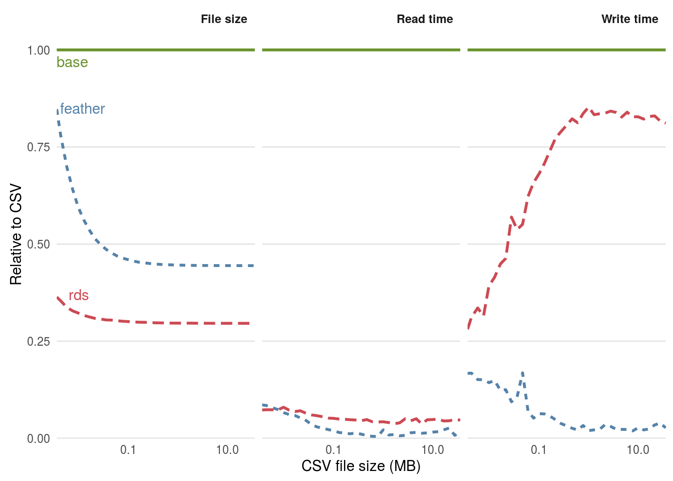
Figure 5.2: Comparison of the performance of binary formats for reading and writing datasets with 20 column with the plain text format CSV. The functions used to read the files were read.csv(), readRDS() and feather::read_feather() respectively. The functions used to write the files were write.csv(), saveRDS() and feather::write_feather().

The results of this simple disk usage benchmark show that saving data in a compressed binary format can save space and if your data will be shared on-line, data download time and bandwidth usage perspectives. But how does each method compare from a computational efficiency perceptive? The read and write times for each file format are illustrated in the middle and right hand panels of 5.2.

The results show that file size is not a reliable predictor of data read and write times. This is due to the computational overheads of compression. Although feather files occupied more disc space, they were roughly equivalent in terms of read times: the functions read_feather() and readRDS() were consistently around 10 times faster than read.csv(). In terms of write times, feather excels: write_feather() was around 10 times faster than write.csv(), whereas saveRDS() was only around 1.2 times faster.

Note that the performance of different file formats depends on the content of the data being saved. The benchmarks above showed savings for matrices of random numbers. For real life data, the results would be quite different. The voyages dataset, saved as an Rds file, occupied less than a quarter the disc space as the original TSV file, whereas the file size was larger than the original when saved as a feather file!

5.4.4 Protocol Buffers

Google’s Protocol Buffers offers a portable, efficient and scalable solution to binary data storage. A recent package, RProtoBuf, provides an R interface. This approach is not covered in this book, as it is new, advanced and not (at the time of writing) widely used in the R community. The approach is discussed in detail in a paper on the subject, which also provides an excellent overview of the issues associated with different file formats (Eddelbuettel, Stokely, and Ooms 2016).

5.5 Getting data from the internet

The code chunk below shows how the functions download.file() and unzip() can be used to download and unzip a dataset from the internet. (Since R 3.2.3 the base function download.file() can be used to download from secure (https://) connections on any operating system.) R can automate processes that are often performed manually, e.g. through the graphical user interface of a web browser, with potential advantages for reproducibility and programmer efficiency. The result is data stored neatly in the data directory ready to be imported. Note we deliberately kept the file name intact help with documentation, enhancing understanding of the data’s provenance, so future users can quickly find out where the data came from. Note also that part of the dataset is stored in the efficient package. Using R for basic file management can help create a reproducible workflow, as illustrated below.

url = "https://www.monetdb.org/sites/default/files/voc_tsvs.zip"
download.file(url, "voc_tsvs.zip") # download file
unzip("voc_tsvs.zip", exdir = "data") # unzip files
file.remove("voc_tsvs.zip") # tidy up by removing the zip file

This workflow equally applies to downloading and loading single files. Note that one could make the code more concise by entering replacing the second line with df = read.csv(url). However, we recommend downloading the file to disk so that if for some reason it fails (e.g. if you would like to skip the first few lines), you don’t have to keep downloading the file over and over again. The code below downloads and loads data on atmospheric concentrations of CO². Note that this dataset is also available from the datasets package.

url = "https://vincentarelbundock.github.io/Rdatasets/csv/datasets/co2.csv"
download.file(url, "extdata/co2.csv")
df_co2 = read_csv("extdata/co2.csv")

There are now many R packages to assist with the download and import of data. The organisation rOpenSci supports a number of these. The example below illustrates this using the WDI package (not supported by rOpenSci) to accesses World Bank data on CO2 emissions in the transport sector:

library("WDI")
WDIsearch("CO2") # search for data on a topic
co2_transport = WDI(indicator = "EN.CO2.TRAN.ZS") # import data

There will be situations where you cannot download the data directly or when the data cannot be made available. In this case, simply providing a comment relating to the data’s origin (e.g. # Downloaded from http://example.com) before referring to the dataset can greatly improve the utility of the code to yourself and others.

There are a number of R packages that provide more advanced functionality than simply downloading files. The CRAN task view on Web technologies provides a comprehensive list. The two packages for interacting with web pages are httr and RCurl. The former package provides (a relatively) user-friendly interface for executing standard HTTP methods, such as GET and POST. It also provides support for web authentication protocols and returns HTTP status codes that are essential for debugging. The RCurl package focuses on lower-level support and is particularly useful for web-based XML support or FTP operations.

5.6 Accessing data stored in packages

Most well documented packages provide some example data for you to play with. This can help demonstrate use cases in specific domains, that uses a particular data format. The command data(package = "package_name") will show the datasets in a package. Datasets provided by dplyr, for example, can be viewed with data(package = "dplyr").

Raw data (i.e. data which has not been converted into R’s native .Rds format) is usually located with the sub-folder extdata in R (which corresponds to inst/extdata when developing packages. The function system.file() outputs file paths associated with specific packages. To see all the external files within the readr package, for example, one could use the following command:

list.files(system.file("extdata", package = "readr"))
#> [1] "challenge.csv"     "compound.log"      "epa78.txt"        
#> [4] "example.log"       "fwf-sample.txt"    "massey-rating.txt"
#> [7] "mtcars.csv"        "mtcars.csv.bz2"    "mtcars.csv.zip"

Further, to ‘look around’ to see what files are stored in a particular package, one could type the following, taking advantage of RStudio’s intellisense file completion capabilities (using copy and paste to enter the file path):

system.file(package = "readr")
#> [1] "/home/robin/R/x86_64-pc-linux-gnu-library/3.3/readr"

Hitting Tab after the second command should trigger RStudio to create a miniature pop-up box listing the files within the folder, as illustrated in figure 5.3.

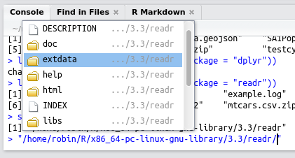
Figure 5.3: Discovering files in R packages using RStudio’s ‘intellisense’.

References

Eddelbuettel, Dirk, Murray Stokely, and Jeroen Ooms. 2016. “RProtoBuf: Efficient Cross-Language Data Serialization in R.” Journal of Statistical Software 71 (1): 1–24. doi:10.18637/jss.v071.i02.

---

14. Geographical data, for example, can be slow to read in external formats. A large .shp or .geojson file can take more than \(100\) times longer to load than an equivalent .Rds or .Rdata file.↩