4.6 Repeated measures ANOVA
In this experiment, we have more than one measure per unit of observation, namely willingness to spend for conspicuous products and willingness to spend for inconspicuous products. A repeated measures ANOVA can be used to test whether the effects of the experimental conditions are different for conspicuous versus inconspicuous products.
To carry out a repeated measures ANOVA, we need to restructure our data frame from wide to long. A wide data frame has one row per unit of observation (in our experiment: one row per participant) and one column per observation (in our experiment: one column for the conspicuous products and one column for the inconspicuous products). A long data frame has one row per observation (in our experiment: two rows per participant, one row for the conspicuous product and one row for the inconspicuous product) and an extra column that denotes which type of observation we are dealing with (conspicuous or inconspicuous). Let’s convert the data frame and then see how wide and long data frames differ from each other.
powercc.long <- powercc %>%
  pivot_longer(cols = c(cc, icc), names_to = "consumption_type", values_to = "wtp")


# Converting from wide to long means that we're stacking a number of columns on top of each other.
# The pivot_longer function converts datasets from wide to long and takes three arguments:
# 1. The cols argument: here we tell R which columns we want to stack. The original dataset had 143 rows with 143 values for conspicuous products in the variable cc and 143 values for inconspicuous products in the variable icc. The long dataset will have 286 rows with 286 values for conspicuous or inconspicuous products. This means we need to keep track of whether we are dealing with a value for conspicuous or inconspicuous products.
# 2. The names_to argument: here you define the name of the variable that keeps track of whether we are dealing with a value for conspicuous or inconspicuous products.
# 3. The values_to argument: here you define the name of the variable that stores the actual values.


# Let's tell R to show us only the relevant columns (this is just for presentation purposes):
powercc.long %>%
  select(subject, power, audience, consumption_type, wtp) %>%
  arrange(subject)
## # A tibble: 286 x 5
## subject power audience consumption_type wtp
## <fct> <fct> <fct> <chr> <dbl>
## 1 1 high public cc 5
## 2 1 high public icc 2.6
## 3 2 low public cc 7.6
## 4 2 low public icc 4
## 5 3 low public cc 5.4
## 6 3 low public icc 3.4
## 7 4 low public cc 8.4
## 8 4 low public icc 5.2
## 9 5 high public cc 7.8
## 10 5 high public icc 3
## # ... with 276 more rowsWe have two rows per subject, one column for willingness to pay and another column (consumption_type) denoting whether it’s willingness to pay for conspicuous or inconspicuous products. Compare this with the wide dataset:
powercc %>%
  select(subject, power, audience, cc, icc) %>%
  arrange(subject) # Show only the relevant columns
## # A tibble: 143 x 5
## subject power audience cc icc
## <fct> <fct> <fct> <dbl> <dbl>
## 1 1 high public 5 2.6
## 2 2 low public 7.6 4
## 3 3 low public 5.4 3.4
## 4 4 low public 8.4 5.2
## 5 5 high public 7.8 3
## 6 6 high public 7.2 5
## 7 7 low public 4.8 4
## 8 8 high public 6.6 4.4
## 9 9 low public 5.8 4.2
## 10 10 high public 6.8 3.4
## # ... with 133 more rowsWe have one row per subject and two columns, one for each type of product.
We can now carry out a repeated measure ANOVA. For this we need the ez package.
install.packages("ez") # We need the ez package for RM Anova
library(ez)
We want to test whether the interaction between power and audience is different for conspicuous and for inconspicuous products. Let’s take a look at a graph first:
powercc.long.summary <- powercc.long %>% # for a bar plot, we need a summary first
  group_by(power, audience, consumption_type) %>% # group by three independent variables
  summarize(wtp = mean(wtp)) # get the mean wtp
## `summarise()` regrouping output by 'power', 'audience' (override with `.groups` argument)ggplot(data = powercc.long.summary, mapping = aes(x = audience, y = wtp, fill = power)) +
facet_wrap(~ consumption_type) + # create a panel for each consumption type
geom_bar(stat = "identity", position = "dodge")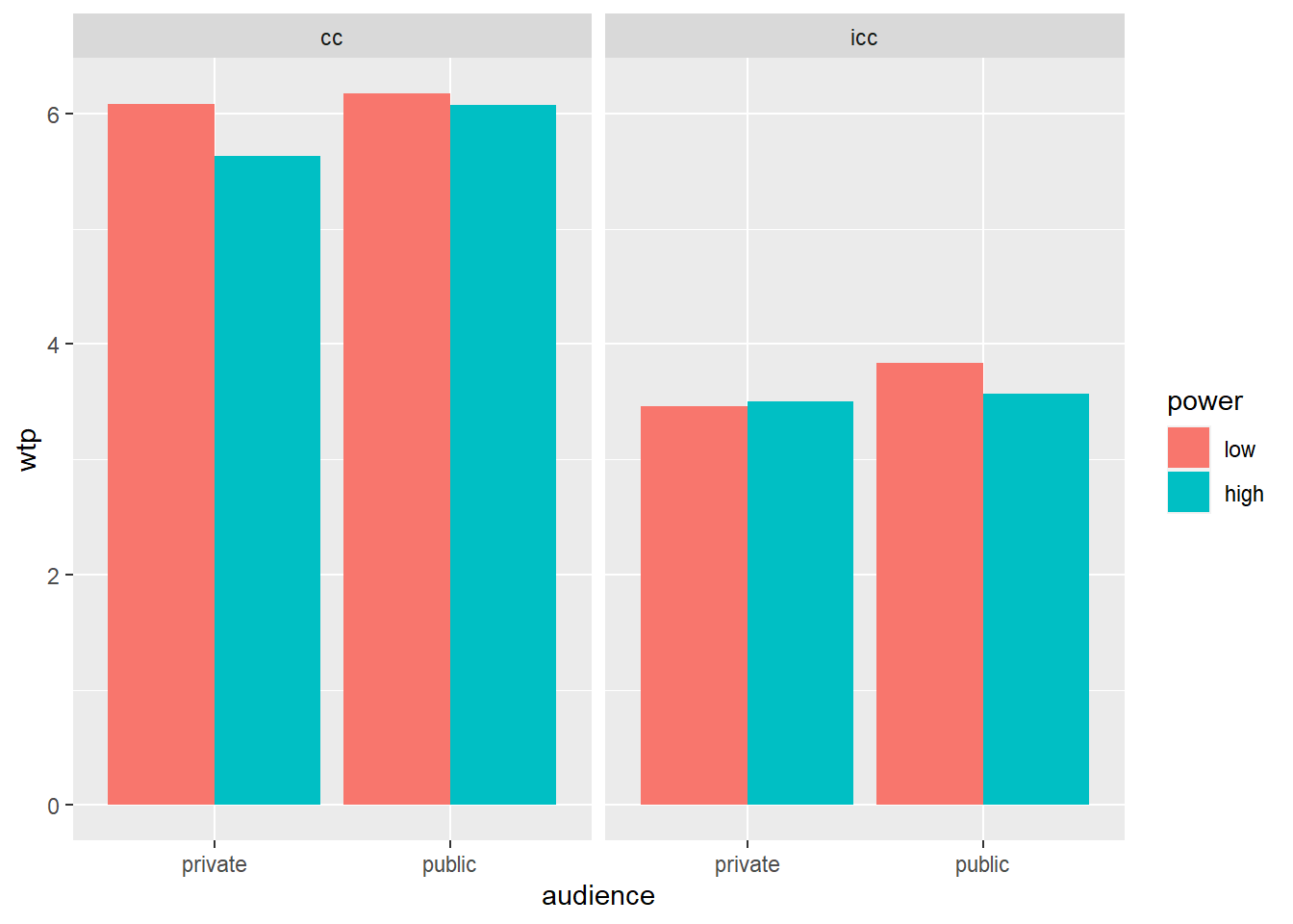
We can now formally test the three-way interaction:
# Specify the data, the dependent variable, the identifier (wid),
# the variable that represents the within-subjects condition, and the variables that represent the between subjects conditions.
ezANOVA(data = powercc.long, dv = wtp, wid = subject, within = consumption_type, between = power*audience)
## $ANOVA
## Effect DFn DFd F p p<.05
## 2 power 1 139 1.867530e+00 1.739647e-01
## 3 audience 1 139 2.977018e+00 8.667716e-02
## 5 consumption_type 1 139 6.303234e+02 1.687352e-53 *
## 4 power:audience 1 139 5.801046e-03 9.393977e-01
## 6 power:consumption_type 1 139 4.719313e-01 4.932445e-01
## 7 audience:consumption_type 1 139 2.700684e-02 8.697041e-01
## 8 power:audience:consumption_type 1 139 2.982598e+00 8.638552e-02
## ges
## 2 9.061619e-03
## 3 1.436772e-02
## 5 5.915501e-01
## 4 2.840440e-05
## 6 1.083172e-03
## 7 6.204919e-05
## 8 6.806406e-03We see in these results that the three-way interaction between power, audience, and consumption type is marginally significant. You can report this as follows: "A repeated measures ANOVA established that the three-way interaction between power, audience, and consumption type, was marginally significant (F(1, 139) = 2.98, p = 0.086).